Using AI for Wavefront Estimation with the Rubin Observatory Active Optics System

Abstract: The Vera C. Rubin Observatory will, over a period of 10 years, repeatedly survey the southern sky. To ensure that images generated by Rubin meet the quality requirements for precision science, the observatory will use an Active Optics System (AOS) to correct for alignment and mirror surface perturbations introduced by gravity and temperature gradients in the optical system. To accomplish this Rubin will use out-of-focus images from sensors located at the edge of the focal plane to learn and correct for perturbations to the wavefront. We have designed and integrated a deep learning model for wavefront estimation into the AOS pipeline. In this paper, we compare the performance of this deep learning approach to Rubin's baseline algorithm when applied to images from two different simulations of the Rubin optical system. We show the deep learning approach is faster and more accurate, achieving the atmospheric error floor both for high-quality images, and low-quality images with heavy blending and vignetting. Compared to the baseline algorithm, the deep learning model is 40x faster, the median error 2x better under ideal conditions, 5x better in the presence of vignetting by the Rubin camera, and 14x better in the presence of blending in crowded fields. In addition, the deep learning model surpasses the required optical quality in simulations of the AOS closed loop. This system promises to increase the survey area useful for precision science by up to 8%. We discuss how this system might be deployed when commissioning and operating Rubin.

• The paper introduces a deep learning model that directly regresses 19 Zernike coefficients from donut images, improving estimation accuracy over traditional TIE methods.
• It leverages a fine-tuned ResNet-18 architecture to reduce FWHM error by ~2x under ideal conditions and shows robust performance in low SNR, vignetting, and blending scenarios.
• The approach enables single-donut wavefront estimation and enhances operational resilience, expanding high-quality sky coverage by approximately 1400 deg².

AI-Based Wavefront Estimation for the Rubin Observatory Active Optics System

Introduction

The Vera C. Rubin Observatory imposes stringent requirements on image quality to enable transformative cosmological and astrophysical studies with the Legacy Survey of Space and Time (LSST). Wavefront sensing and control is central to achieving these requirements due to the complexity and scale of the optical system. Traditional wavefront estimation within Rubin’s Active Optics System (AOS) is based on solving the transport of intensity equation (TIE) from out-of-focus stellar images (“donuts”). This work introduces, implements, and benchmarks a deep learning (DL) model for direct Zernike coefficient regression from donut images, with the aim of improving speed, robustness, and accuracy of wavefront estimation under real-world observational challenges (e.g., blending, vignetting, and variable SNR).

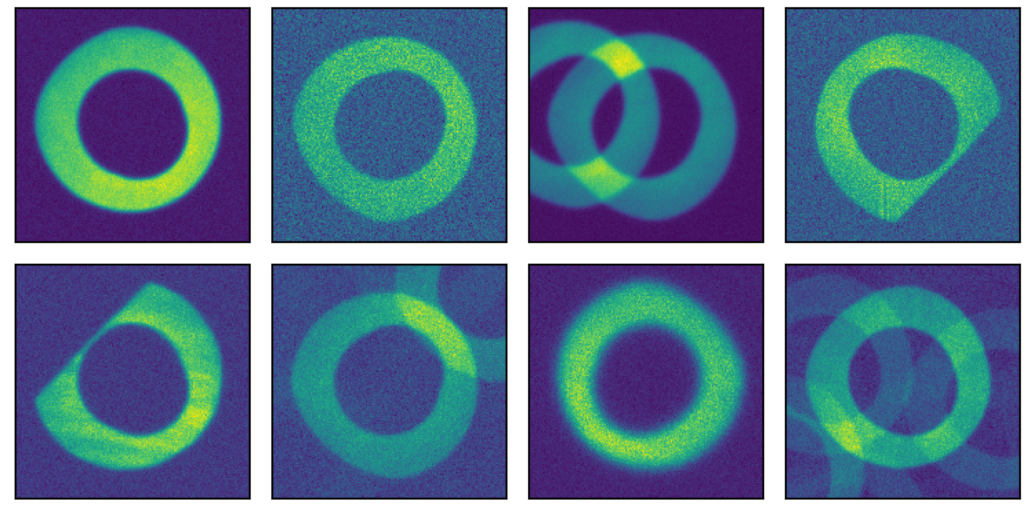
Figure 1: Example donut images simulated with Batoid and GalSim, demonstrating diversity in SNR, vignetting, and source blending.

Simulation and Data Preparation

Simulated training, validation, and test datasets are generated using high-fidelity optical simulations (Batoid and GalSim) incorporating realistic stellar catalogs, atmospheric effects, instrumental vignetting, blending, and a range of optical aberrations parameterized by Zernike polynomials. The test regime encompasses both ideal (isolated, unvignetted, high-SNR) and degraded (blending, vignetting, low-SNR) conditions, thereby exposing the ML model and baseline TIE to the full operational envelope.

Deep Learning Estimator Architecture

The DL model leverages a convolutional neural network (CNN) base, specifically a fine-tuned ResNet-18 architecture pretrained on ImageNet, followed by a fully-connected head. The input consists of a single donut image and metadata: intra/extra-focal flag, field angle, and effective wavelength. The network is trained to directly regress 19 Zernike coefficients (Noll indices 4–22) with a loss weighted to minimize the PSF FWHM degradation contributed by Zernike residuals, yielding a loss proxy directly matched to survey requirements.

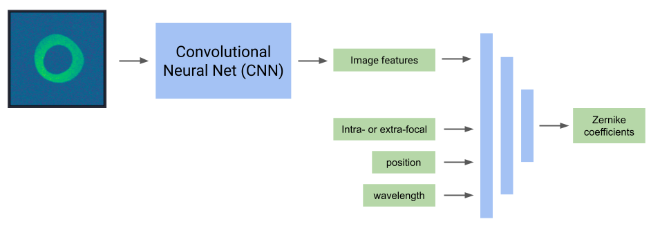
Figure 2: Architecture schematic: donut image processed by CNN, concatenated with metadata, and mapped by the head to Zernike amplitudes.

Comparison with Baseline TIE Solver

Individual Example and Statistical Performance

Qualitative behavior is illustrated with individual intra/extra-focal pairs, revealing that in ideal conditions, the DL estimator’s output matches simulated truth to within atmospheric noise, while the TIE solution exhibits systematic deviations even when classical assumptions are approximately satisfied.

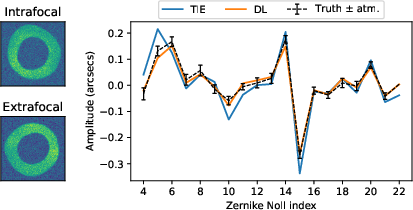
Figure 3: Individual intra/extra-focal donut processed by both AOS pipeline methods, showing DL and TIE Zernike estimates vs. ground truth.

Quantitatively, the DL model achieves a median FWHM degradation error $\sim$2x lower than TIE in ideal conditions. The full distribution is consistent with the irreducible atmospheric error floor, while TIE errors are offset and fail to meet the required $0.079''$ criterion except in a negligible fraction of cases.

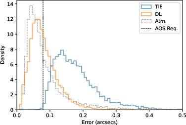
Figure 4: Error distributions for both methods under ideal conditions; DL is statistically limited by atmospheric randomness, TIE does not reach this limit.

Sensitivity to SNR, Vignetting, and Blending

Wavefront estimation error escalates for both methods below SNR$\sim$200, but the progression is more gradual for DL, which matches TIE performance at SNR$>$200 despite using a fundamentally different algorithmic approach.

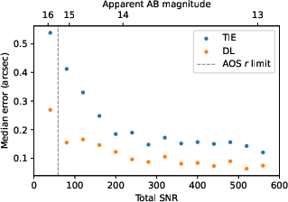
Figure 5: Median estimation error versus SNR, showing DL resilience down to lower SNR than TIE.

Camera vignetting (edge-of-field) severely degrades TIE accuracy (increase by factor of 5 in median error), but has negligible effect on the DL model, which incorporates such effects implicitly during training.

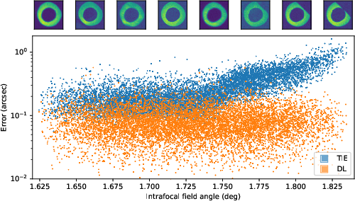
Figure 6: Error as a function of field angle and vignetting. Above 1.74 deg vignetting sharply increases TIE error, not DL error.

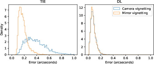
Figure 7: TIE and DL error distributions split by vignetting regime; DL's performance is invariant, TIE's is severely impacted for vignetted sources.

Blending (coincident or nearby sources) catastrophically corrupts the TIE solution (increase by factor of 14 in some regimes; frequent outright failures). The DL estimator is robust to both bright and faint blends, with only a modest degradation in extreme cases.

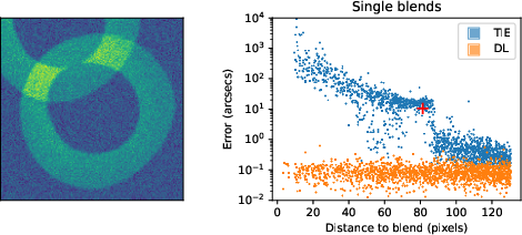
Figure 8: The impact of bright blending as a function of blend distance: the DL maintains accuracy, TIE rapidly degrades.

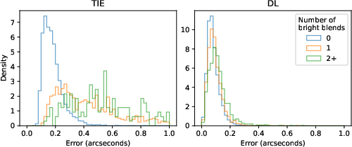
Figure 9: Error distributions by number of bright blends: TIE fails frequently with multiple blends, DL degrades gracefully.

Blending by faint sources only modestly increases DL error, with no significant effect seen until a substantial number of moderate blends are present.

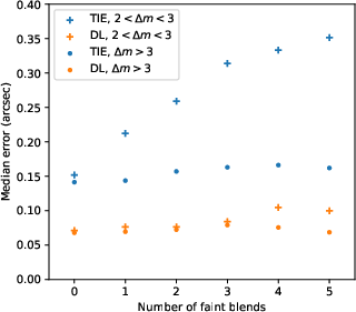
Figure 10: Median DL/TIE errors as a function of faint blend count. DL is less sensitive than TIE and only mildly degrades under stacking faint blends.

Integration and End-to-End Closed Loop Performance

The DL model is evaluated on full AOS closed-loop simulations where wavefront estimation is coupled with the optical control feedback. On high-fidelity PhoSim data (distinct from Batoid training set), the DL model achieves requirement-level PSF FWHM and PSSN (both metrics converging across iterations), attesting to absence of overfitting. The DL and TIE methods both deliver similar ultimate performance, but the DL model is modestly superior in final PSF width and stability.

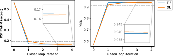
Figure 11: Closed-loop PSF FWHM and PSSN convergence for TIE/DL estimators; DL achieves slightly better final metrics.

Single-Sided Estimation and Implications

A notable advantage of the DL model is the ability to estimate the wavefront using only a single donut from either the intra- or extra-focal side, with no significant penalty to accuracy. Statistical distributions of estimation error are nearly identical whether pairs are intra/extra, intra/intra, or extra/extra, a result that is unattainable for the TIE solver.

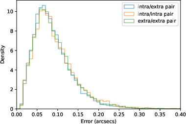
Figure 12: DL model error distributions for intra/extra, intra/intra, and extra/extra pairs; all three overlap, supporting single-donut estimation.

This property enhances operational resilience in the presence of sensor failures, poor source pairing, or fields with dominated vignetting/blending on one side.

Performance and Scalability Considerations

The DL model is 40x faster at inference per donut-pair than the TIE solver using standard hardware. Moreover, unlike the TIE algorithm, inference over many independent donuts can be trivially batched, with further speedup as a function of available computational resources. Training remains offline and computationally intensive, but this cost is negligible on operational timescales.

Implications for Rubin AOS and Broader Context

The DL wavefront estimator enables reliable AOS operation in the $\sim$8% of fields where TIE fails, expanding the high-quality, science-grade sky area by $\sim$1400 deg$^2$. It also increases the diversity of wavefront sensor usage, provides immunity to classically problematic observing configurations (crowded or vignetted regions), and maintains survey efficiency by reducing computational bottlenecks.

Current limitations include the necessity for adequate domain transfer—ensuring performance on real data despite potentially unmodeled effects in simulation. The authors suggest explicit domain adaptation strategies (such as adversarial feature adaptation) and the generation of even more comprehensive simulation suites to span the true range of instrumental and physical conditions.

Conclusion

This work demonstrates that a supervised DL system trained on a comprehensive and realistic simulation set can directly infer wavefront Zernike coefficients from individual donut images, attaining performance statistically indistinguishable from the atmospheric error floor under optimal conditions, and significantly outperforming the baseline TIE solver in the presence of vignetting, blending, or low SNR. The model generalizes to independent simulation pipelines and supports robust closed-loop optical control. Its computational efficiency and operational flexibility substantially enhance Rubin AOS capabilities and provide a working template for similarly challenging wavefront inference tasks in future large survey facilities.

Future directions include large-scale, on-sky validation, development of unsupervised or semi-supervised domain adaptation pipelines, and systematic investigation of model generalization properties under further-realistic instrument artifacts and hardware failures. This research illustrates both the necessity and the efficacy of machine learning approaches for real-time, robust, and scalable wavefront control in next-generation astrophysical instrumentation.