Dynamic Investment Strategies Through Market Classification and Volatility: A Machine Learning Approach

Abstract: This study introduces a dynamic investment framework to enhance portfolio management in volatile markets, offering clear advantages over traditional static strategies. Evaluates four conventional approaches : equal weighted, minimum variance, maximum diversification, and equal risk contribution under dynamic conditions. Using K means clustering, the market is segmented into ten volatility-based states, with transitions forecasted by a Bayesian Markov switching model employing Dirichlet priors and Gibbs sampling. This enables real-time asset allocation adjustments. Tested across two asset sets, the dynamic portfolio consistently achieves significantly higher risk-adjusted returns and substantially higher total returns, outperforming most static methods. By integrating classical optimization with machine learning and Bayesian techniques, this research provides a robust strategy for optimizing investment outcomes in unpredictable market environments.

• The paper presents a dynamic portfolio framework that integrates K-means clustering, Bayesian Markov switching, and classical optimization to adjust asset allocation in real time.
• It employs market segmentation into 10 volatility states and uses Gibbs sampling to estimate state transition probabilities for improved decision making.
• Empirical results indicate that the proposed strategy outperforms static methods, achieving significantly higher total returns and Sharpe ratios across diverse asset sets.

Dynamic Investment Strategies via Machine Learning

This paper introduces a dynamic investment framework that enhances portfolio management in volatile markets. It addresses the limitations of traditional static strategies by integrating K-means clustering, Bayesian Markov switching models, and classical portfolio optimization techniques. The approach categorizes market states based on volatility and dynamically adjusts asset allocation to optimize risk-adjusted returns.

Methodology

The methodology consists of three key steps: market segmentation using K-means clustering, transition modeling via a Bayesian Markov switching model, and dynamic portfolio construction using classical portfolio optimization methods.

K-Means Clustering for Market Segmentation

The paper segments historical market volatility into ten distinct states using the K-means clustering algorithm. This approach identifies regimes of low, medium, and high volatility by minimizing the within-cluster sum of squares (WCSS).

The K-means algorithm partitions $n$ observations into $k$ clusters, aiming to minimize the WCSS, which is defined as:

$$\text{WCSS} = \sum_{i=1}^{k} \sum_{x \in C_i} \| x - \mu_i \|^2,$$

where $C_i$ represents the set of observations in cluster $i$ and $\mu_i$ is the mean of the observations in cluster $i$. This segmentation provides a granular view of how different portfolio strategies perform under varying market conditions.

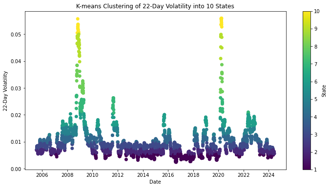
Figure 1: K-means Clustering of 22-Day Volatility into 10 States for SPY Top 11 Portfolio.

Bayesian Markov Switching Model

To model the transitions between the identified market states, the paper employs a Bayesian approach to estimate the transition probabilities. This method incorporates prior knowledge through a Dirichlet prior and uses Markov Chain Monte Carlo (MCMC) methods, specifically Gibbs sampling, to derive the transition probabilities. The Dirichlet prior, known for its conjugacy with the Multinomial distribution, is suitable for modeling probability vectors that sum to 1. The concentration parameters for the Dirichlet distribution, representing prior counts for transitions from each Markov state, are denoted as:

$$\alpha_{i} = (\alpha_{i1}, \alpha_{i2}, \dots, \alpha_{i10})$$

Here, $\alpha_{ij}$ represents the prior belief about the transition from Markov state $i$ to state $j$. The posterior distribution for the transition probabilities is given by the Dirichlet distribution:

$$P_i = (P_{i1}, P_{i2}, \dots, P_{i10}) \sim \text{Dirichlet}(\alpha_{i1} + N_{i1}, \alpha_{i2} + N_{i2}, \dots, \alpha_{i10} + N_{i10}),$$

where $N_{ij}$ is the number of transitions from state $i$ to state $j$. Gibbs sampling is then used to iteratively refine the posterior distribution. The mixing time, crucial for assessing the convergence of the Markov chain, is bounded using the second-largest eigenvalue modulus (SLEM) of the transition matrix $P$.

Portfolio Optimization and Dynamic Allocation

The paper evaluates four distinct portfolio allocation strategies: equally-weighted investment, minimum variance, equal risk contribution (ERC), and maximum diversification. The equally-weighted investment strategy assigns an equal proportion of the total investment to each asset. The minimum variance portfolio aims to minimize the overall variance of the portfolio, while the maximum diversification strategy maximizes the diversification ratio. The ERC portfolio allocates weights such that each asset contributes equally to the overall portfolio risk.

The dynamic portfolio strategy combines these methods by allocating weights based on the state probabilities derived from the Bayesian Markov switching model. The total return weights for each method are calculated using the transition matrix and vectors representing the optimal return methods for each state.

Empirical Results

The empirical analysis uses daily adjusted closing prices from two asset sets. The first set includes 11 major companies spanning from June 20, 2005, to June 20, 2024, representing the top stocks of 11 sectors of the S{content}P 500 as of June 20, 2024. The second asset set includes NASDAQ, SPY, Bitcoin, Gold, and the iShares 20+ Year Treasury Bond ETF (TLT) spanning from January 6, 2015, to June 20, 2024. The results demonstrate that the dynamic portfolio strategy achieved competitive performance relative to static investment strategies. For the first asset set, the dynamic portfolio achieved a total return of 4910\% and a Sharpe ratio of 237.90. For the second asset set, the dynamic portfolio achieved a total return of 5993\% and a Sharpe ratio of 47.60. The total return weights calculated for each method for the first and second asset sets are shown in tables in the paper.

Discussion and Implications

The results suggest that the dynamic portfolio strategy can adapt to changing market conditions by leveraging the Bayesian Markov transition matrix and dynamically allocating weights based on the best return methods for each state. In particular, a higher correlation among assets in the first set of assets was found to lead to better performance results, highlighting the importance of asset selection in the construction of a diversified portfolio.

Conclusion

The paper concludes that the dynamic portfolio strategy shows significant promise in improving returns and Sharpe ratios through better future state prediction and adaptation. However, it also identifies several areas for future research, such as incorporating additional macroeconomic and financial factors, exploring alternative models, and expanding the analysis to include a broader range of assets. These enhancements could further improve the strategy's practical applicability across diverse market conditions.