A Bayesian Dirichlet Auto-Regressive Conditional Heteroskedasticity Model for Compositional Time Series

Abstract: We analyze daily Airbnb service-fee shares across eleven settlement currencies, a compositional series that shows bursts of volatility after shocks such as the COVID-19 pandemic. Standard Dirichlet time series models assume constant precision and therefore miss these episodes. We introduce B-DARMA-DARCH, a Bayesian Dirichlet autoregressive moving average model with a Dirichlet ARCH component, which lets the precision parameter follow an ARMA recursion. The specification preserves the Dirichlet likelihood so forecasts remain valid compositions while capturing clustered volatility. Simulations and out-of-sample tests show that B-DARMA-DARCH lowers forecast error and improves interval calibration relative to Dirichlet ARMA and log-ratio VARMA benchmarks, providing a concise framework for settings where both the level and the volatility of proportions matter.

• The paper introduces a Bayesian DARCH model that integrates a dynamic precision parameter to capture volatility clustering in compositional time series.
• It employs an ALR-VARMA framework for mean dynamics combined with a stochastic DARCH process, leading to significant improvements in forecast accuracy.
• Empirical and simulation studies show reduced forecast errors and lower residual autocorrelation, validating the model's effectiveness in volatile environments.

Bayesian Dirichlet Auto-Regressive Conditional Heteroskedasticity for Compositional Time Series

Introduction and Motivation

The paper introduces the Bayesian Dirichlet Auto-Regressive Moving Average with Dirichlet Auto-Regressive Conditional Heteroskedasticity (B-DARMA-DARCH) model, targeting the modeling and forecasting of compositional time series with time-varying volatility. The motivating application is Airbnb’s daily currency-fee proportions, a high-frequency compositional dataset where each observation is a vector of non-negative proportions summing to one. These data exhibit both strong temporal dependence and pronounced volatility clustering, especially during periods of market disruption such as the COVID-19 pandemic.

Traditional approaches for compositional time series, such as log-ratio transformed VARMA models or Dirichlet ARMA models with constant or deterministic precision, are inadequate for capturing the observed heteroskedasticity and volatility clustering. The B-DARMA-DARCH model addresses these limitations by introducing a stochastic, time-varying precision parameter via a DARCH (Dirichlet Auto-Regressive Conditional Heteroskedasticity) process, analogous to GARCH for real-valued time series, but adapted to the simplex.

Model Specification

Dirichlet Data Model

Let $\mathbf{y}_t \in \mathcal{S}^{J-1}$ denote the $J$-component compositional observation at time $t$. The model assumes

$$\mathbf{y}_t \mid \boldsymbol{\mu}_t, \phi_t \sim \operatorname{Dirichlet}(\phi_t \boldsymbol{\mu}_t)$$

where $\boldsymbol{\mu}_t$ is the mean vector (on the simplex) and $\phi_t$ is the precision parameter controlling the concentration.

Mean Dynamics via ALR-VARMA

The mean vector is parameterized through the additive log-ratio (ALR) transformation, mapping the simplex to $\mathbb{R}^{J-1}$. The transformed mean, $$\boldsymbol{\eta}_t = \operatorname{alr}(\boldsymbol{\mu}_t)$$, is modeled as a VARMA process:

$$\boldsymbol{\eta}_t = \sum_{p=1}^P \mathbf{A}_p (\operatorname{alr}(\mathbf{y}_{t-p}) - \mathbf{X}_{t-p}\boldsymbol{\beta}) + \sum_{q=1}^Q \mathbf{B}_q (\operatorname{alr}(\mathbf{y}_{t-q}) - \boldsymbol{\eta}_{t-q}) + \mathbf{X}_t \boldsymbol{\beta}$$

where $\mathbf{X}_t$ encodes exogenous covariates (e.g., trend, seasonality).

DARCH Volatility Component

The key innovation is the DARCH process for the precision parameter:

$$\log(\phi_t) = \sum_{l=1}^L \alpha_l (\log(\phi_{t-l}) - \mathbf{z}_{t-l}^\top \boldsymbol{\gamma}) + \sum_{k=1}^K \tau_k \| \mathbf{y}_{t-k} - \boldsymbol{\eta}_{t-k} \|^2 + \mathbf{z}_t^\top \boldsymbol{\gamma}$$

where $\alpha_l$ and $\tau_k$ are AR and MA coefficients, and $\mathbf{z}_t$ are covariates. This recursion allows $\phi_t$ to respond dynamically to both past volatility and recent innovations, capturing volatility clustering and regime shifts.

Simulation Studies

The paper presents six simulation studies to benchmark B-DARMA-DARCH against B-DARMA (with deterministic or constant $\phi_t$) and Bayesian tVARMA (normal VARMA on ALR-transformed data). The studies include both shock scenarios (misreported observations) and regime shifts (parameter changes).

Key findings:

• B-DARMA-DARCH consistently achieves the lowest forecast RMSE and MAE across all scenarios.
• In DARCH DGP settings, B-DARMA-DARCH outperforms B-tVARMA by 12.6% (FRMSE) and 7.7% (FMAE) in shock scenarios, and by 4.7% and 4.6% in regime shift scenarios.
• PACF analysis of standardized squared residuals shows that B-DARMA-DARCH yields substantially lower residual autocorrelation beyond lag 1, indicating superior volatility modeling.

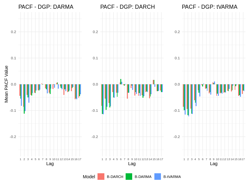
  Figure 1: B-DARMA-DARCH exhibits lower PACF values beyond lag 1, indicating reduced residual autocorrelation and improved volatility capture in simulated compositional time series.

  

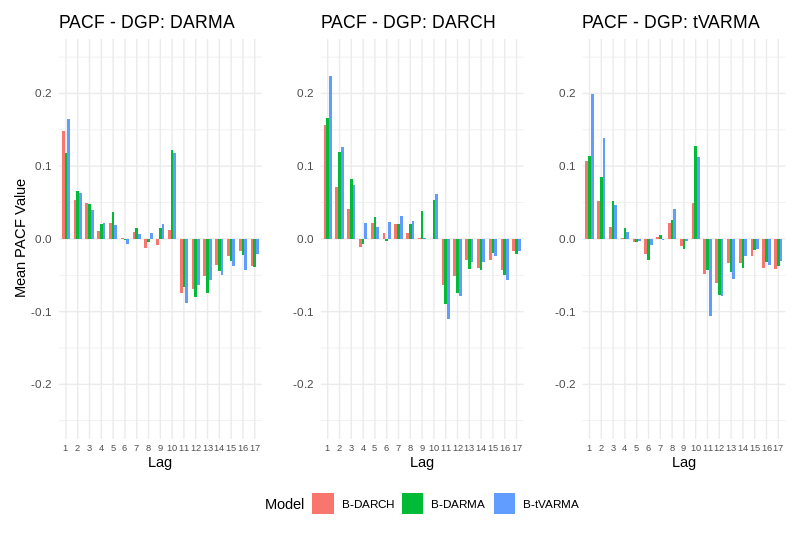
  Figure 2: In regime shift simulations, B-DARMA-DARCH maintains lower residual autocorrelation at higher lags compared to B-DARMA and B-tVARMA.

Empirical Application: Airbnb Currency Fee Proportions

Data and Exploratory Analysis

The empirical study uses Airbnb’s daily currency-fee proportions from 2017–2020, partitioned into four regions, each with six currency categories. The data display strong seasonality, multi-year trends, and volatility clustering, especially during the COVID-19 period.

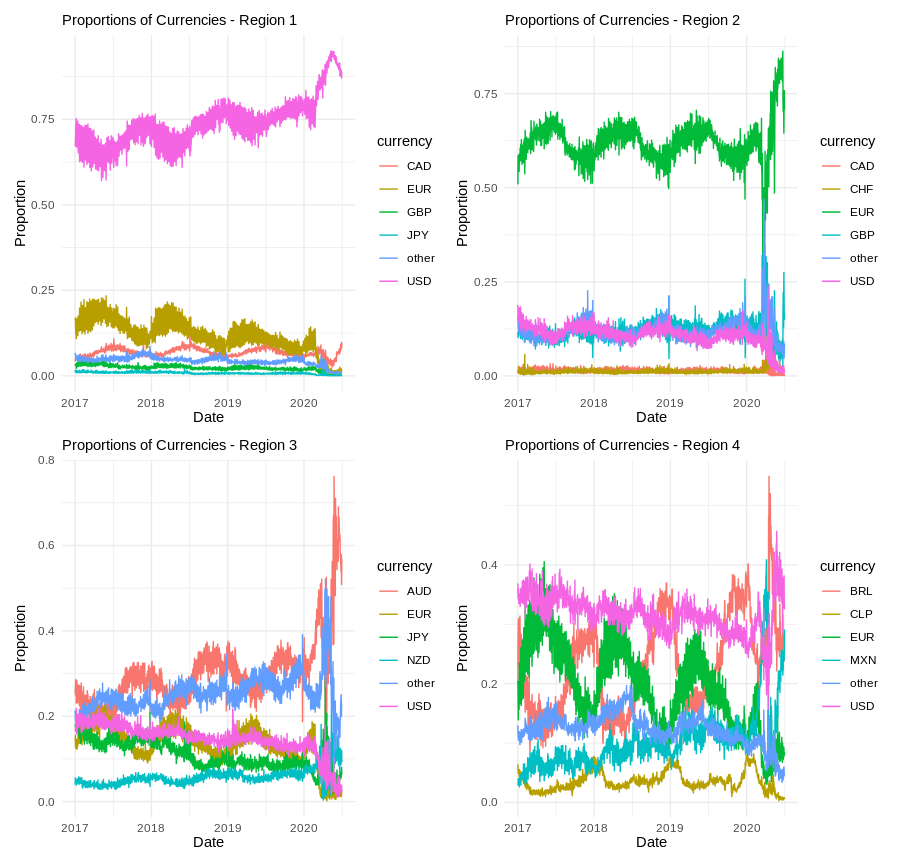
Figure 3: Proportion of fees by billing currency for four regions, illustrating compositional structure and temporal dynamics.

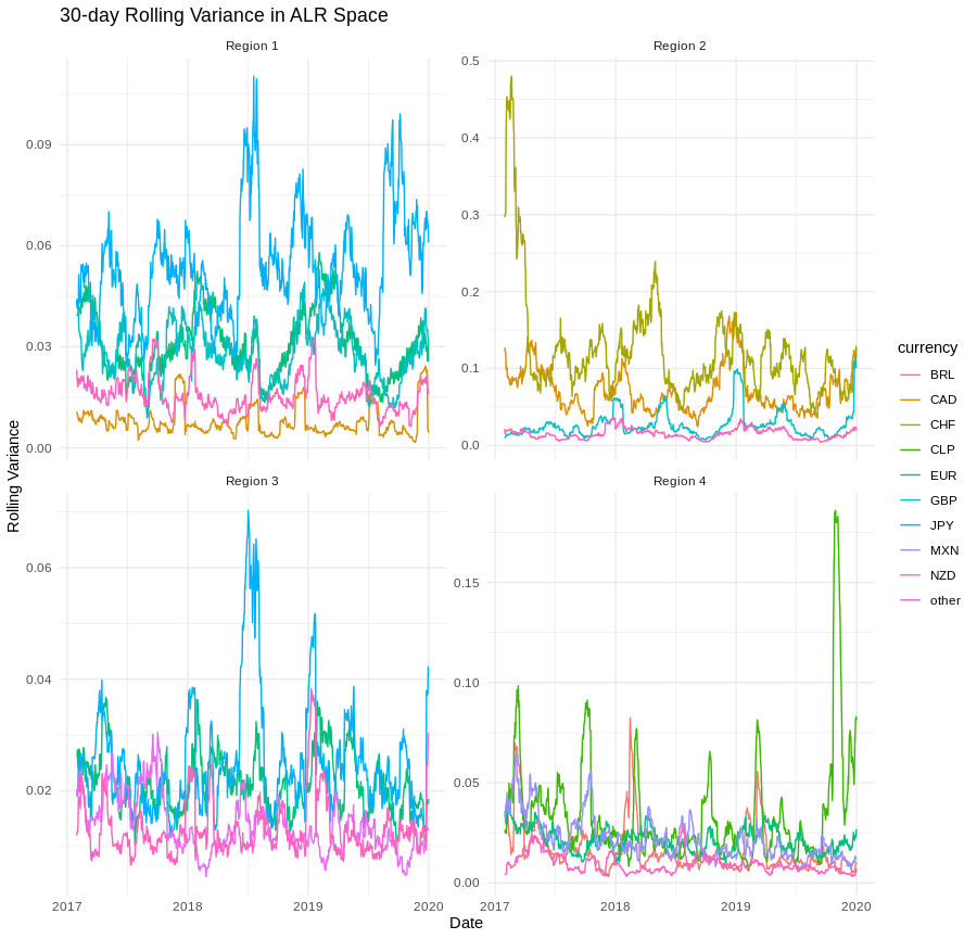
Figure 4: 30-day rolling ALR variance for four regions, highlighting periods of elevated volatility and clustering.

Model Fitting and Validation

All models are fit in a Bayesian framework using Stan, with careful prior specification and inclusion of trend and seasonal covariates (Fourier terms for weekly and yearly cycles). Model selection is performed via validation on a hold-out set, optimizing ARMA orders and seasonal complexity.

Forecasting Results

On the test set (Q4 2020), B-DARMA-DARCH consistently delivers the lowest aggregate FMAE and FRSS across all regions. For example, in Region 1, B-DARMA-DARCH achieves a total FMAE of 2.84, compared to 7.65 (B-DARMA) and 5.20 (B-tVARMA). Coverage of 95% credible intervals is also closest to nominal for B-DARMA-DARCH, with mean coverage rates of 0.92, 0.91, 0.87, and 0.91 across the four regions.

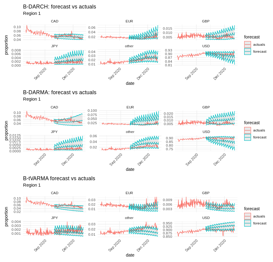
Figure 5: Region 1, 92-day forecasts with 95% confidence intervals for six currencies; B-DARMA-DARCH adapts to volatility and tracks observed values closely.

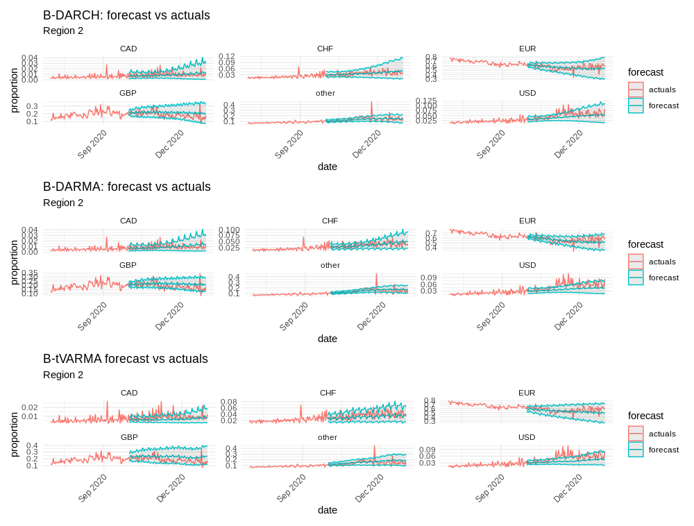
Figure 6: Region 2, 92-day forecasts; B-DARMA-DARCH maintains interval coverage and adapts to abrupt changes.

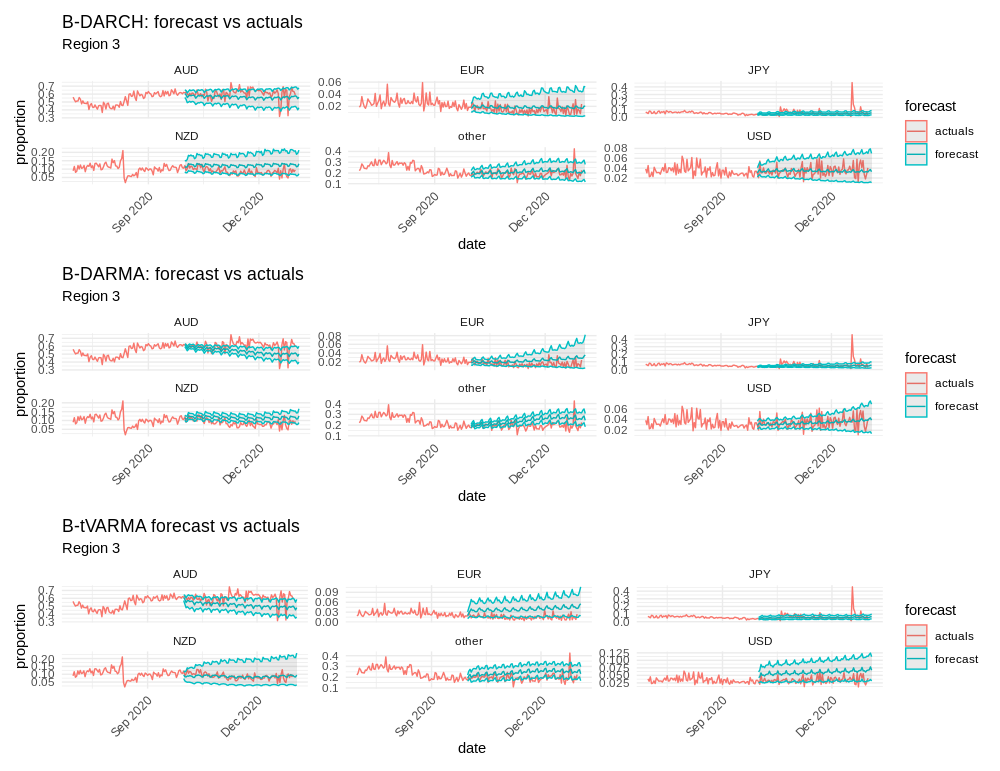
Figure 7: Region 3, 92-day forecasts; B-DARMA-DARCH demonstrates robust adaptation to multi-currency volatility.

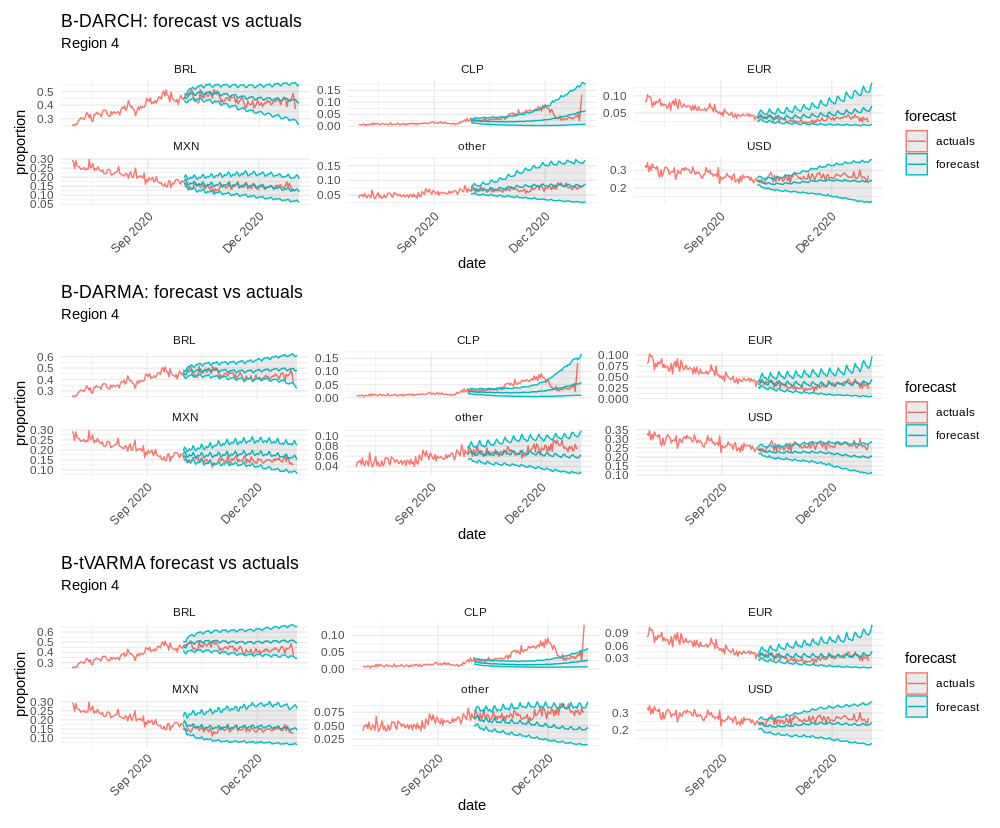
Figure 8: Region 4, 92-day forecasts; B-DARMA-DARCH captures both trend and volatility shifts.

Residual Diagnostics

PACF of standardized squared residuals on the test set confirms that B-DARMA-DARCH achieves minimal residual autocorrelation beyond lag 1, indicating effective volatility modeling. In contrast, B-DARMA and B-tVARMA exhibit persistent autocorrelation at higher lags.

Parameter Interpretation

Posterior densities of DARCH coefficients reveal region-specific volatility regimes. Regions 2 and 3 exhibit high AR coefficients ($\alpha$), indicating persistent volatility, while Region 4 shows a more complex, multi-lag structure with moderate or delayed response.

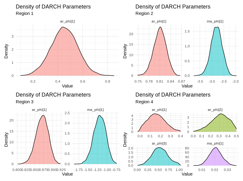
Figure 9: Posterior densities of DARCH model coefficients; high $\alpha$ in Regions 2 and 3 indicate persistent volatility, while Region 4 shows moderate or delayed response.

Theoretical and Practical Implications

The B-DARMA-DARCH model advances the state of compositional time series analysis by:

• Providing a fully Bayesian, simplex-respecting framework for both mean and volatility dynamics.
• Enabling robust uncertainty quantification and risk assessment in settings with volatility clustering and regime shifts.
• Demonstrating empirical superiority in both simulation and real-world financial data, with improved forecast accuracy and interval coverage.

The model’s flexibility allows for the inclusion of exogenous covariates and complex seasonal structures, making it suitable for a wide range of applications in finance, economics, and other domains involving compositional data.

Limitations and Future Directions

The primary limitation is computational: the model’s complexity and the need for MCMC sampling increase resource requirements and necessitate careful tuning for convergence. The current approach models each region independently, ignoring potential cross-region dependencies for shared currencies. Future work could extend the framework to hierarchical or multi-level models, incorporate zero-inflation, or develop scalable approximate inference methods (e.g., variational Bayes).

Conclusion

The B-DARMA-DARCH model provides a principled, flexible, and empirically validated approach for modeling compositional time series with dynamic volatility. Its ability to capture both mean and heteroskedasticity dynamics on the simplex, combined with robust Bayesian inference, makes it a valuable tool for forecasting, risk management, and uncertainty quantification in compositional domains. The methodology is broadly applicable and sets a new standard for compositional time series analysis under volatility.