A Two-Gauge Field Model for Magnetoelectric Boundaries

Abstract: This work introduces a field-theoretical model designed to simulate the presence of material layers with magnetoelectric properties. The model comprises the standard Maxwell field coupled to a Chern-Simons field confined to a planar layer. The electromagnetic behavior of the boundary is emulated through the interaction between the Chern-Simons and Maxwell fields, governed by two parameters: the Chern-Simons mass and the coupling constant between the fields. Both parameters can be adjusted to reflect the specific properties of different materials. We compute the exact propagator of the theory and employ it to investigate several physical properties. Our analysis focuses on phenomena that arise from the presence of external sources coupled to both the Maxwell and Chern-Simons fields, considering various scenarios. In the Chern-Simons sector, the sources emulate defects in the crystal lattice of the material layer. The main objective of this paper is to present the proposed model and to explore its behavior in the simple context of a single planar material interface. We also suggest possible extensions of the model to more general configurations.

• The paper introduces a two-gauge field model that couples the Maxwell field with a planar Chern-Simons field, enabling precise control over magnetoelectric boundary effects via two tunable parameters.
• It derives an exact propagator and interaction energy formulas, revealing how the system transitions between decoupled and strong coupling limits, including standard perfect conductor behavior.
• The findings offer a versatile framework for analyzing electromagnetic phenomena such as induced polarization, forces, and topological interactions in advanced materials.

Two-Gauge Field Model for Magnetoelectric Boundaries: A Field-Theoretic Analysis

Introduction and Motivation

The paper introduces a field-theoretical framework for modeling planar material layers with magnetoelectric properties by coupling the standard Maxwell field to a Chern-Simons (CS) gauge field confined to a plane. The model is constructed in $(3+1)$-dimensional Minkowski space, with the planar CS field localized at $x^3 = a$. The coupling between the bulk Maxwell field and the planar CS field is implemented via a Chern-Simons-like term, parameterized by a coupling constant $\mu$, while the CS field itself is endowed with a mass parameter $m$. This construction allows for two independent tunable parameters, in contrast to previous models that typically feature a single free parameter for boundary effects.

The motivation for this approach is twofold: (i) to provide a more versatile and physically accurate description of magnetoelectric boundaries, and (ii) to enable the study of electromagnetic phenomena not only on the material surface but also in its vicinity, including the effects of external sources and lattice defects. The model generalizes previous $(2+1)$-dimensional treatments by embedding the planar system in a fully dynamical $(3+1)$-dimensional electromagnetic environment.

Model Formulation and Propagator Structure

The Lagrangian density is given by: $$\mathcal{L} = -\frac{1}{4}F^{\mu\nu}F_{\mu\nu} - J_\mu A^\mu - \frac{1}{2\alpha}(\partial_\mu A^\mu)^2 + \left[ -\frac{1}{4}G^{\mu\nu}G_{\mu\nu} - \mathcal{J}_\mu \mathcal{A}^\mu - \frac{1}{2\beta}(\partial_\mu \mathcal{A}^\mu)^2 + \frac{m}{2}\epsilon^{\mu\nu\alpha 3}\mathcal{A}_\mu\partial_\nu \mathcal{A}_\alpha - \frac{\mu}{4}\epsilon^{\mu\nu\alpha 3}(A_\mu\partial_\nu \mathcal{A}_\alpha + \mathcal{A}_\mu\partial_\nu A_\alpha) \right]\delta(x^3 - a)$$ where $A^\mu$ is the Maxwell field, $\mathcal{A}^\mu$ is the planar CS field, $m$ is the CS mass, and $\mu$ is the coupling constant.

The equations of motion reveal that the Maxwell and CS fields are coupled only at the plane $x^3 = a$, with the coupling mediated by the $\delta$-function. The presence of the planar field induces effective polarization and magnetization terms in the Maxwell equations, which can be interpreted as surface responses.

The propagator for the coupled system is derived exactly in matrix form, with the full Green's function $G_{\nu\sigma}(x, y)$ expressed as a sum of the free (uncoupled) propagators and a correction term $\Delta \mathcal{G}_{\nu\sigma}$ that encodes the effects of the CS coupling. The correction term is nontrivial and involves the inversion of a momentum-dependent matrix, reflecting the interplay between the two gauge sectors.

In the strong coupling limit ($\mu \to \infty$), the model reduces to Maxwell electrodynamics with a perfectly conducting boundary at $x^3 = a$, and the CS sector becomes non-propagating. In the decoupling limit ($\mu \to 0$), the two fields evolve independently.

Interaction Energies and Forces

Point Charge–Plane Interaction

The interaction energy between a stationary point charge and the planar potential is computed using the exact propagator. The result is: $$E_{Q\mu}(Q, \mu, m, R_\perp) = -\frac{Q^2 \mu^2 e^{\frac{1}{4} R_\perp \mu^2}}{64\pi} \operatorname{Re}\left\{ e^{2imR_\perp} \Gamma\left[0, \frac{R_\perp}{4}(\mu^2 + 8im)\right] \right\}$$ where $R_\perp$ is the distance from the charge to the plane, and $\Gamma$ is the incomplete Gamma function.

The corresponding force is obtained by differentiating the energy with respect to $R_\perp$. The interaction is always attractive and decays more slowly than the Coulomb force at short distances, but is suppressed at large $R_\perp$ by the parameters $m$ and $\mu$. In the strong coupling limit, the result reduces to the standard image charge interaction for a perfect conductor: $$E_{Q\mu}(Q, \mu = \infty, m, R_\perp) = -\frac{Q^2}{16\pi R_\perp}$$

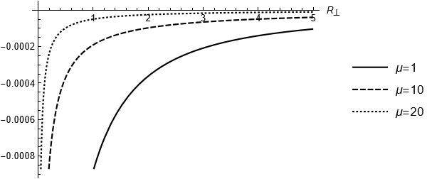
Figure 1: Energy $E_{Q\mu}$ as a function of $R_\perp$ for various $\mu$, showing the crossover from magnetoelectric to perfect conductor behavior.

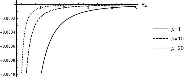
Figure 2: Force $F_{Q\mu}$ as a function of $R_\perp$ for various $\mu$, illustrating the suppression of the interaction with increasing $\mu$.

Planar Source–Source Interactions

The model allows for the computation of interaction energies between various types of sources:

• Two point-like charges in the CS sector: The energy is given in terms of Struve and Neumann functions with complex arguments, leading to an exponentially decaying interaction at large distances. In the decoupling limit, the result reduces to the standard Maxwell-Chern-Simons interaction in $(2+1)$D.

  Figure 3: Energy between two planar CS charges as a function of in-plane separation for different $\mu$.

• Mixed sector (Maxwell–CS) interaction: The energy between a point charge in the Maxwell sector and a point source in the CS sector is

$$E_{Qq}(m, \mu, R_\perp, R_\parallel) = \frac{qQm\mu}{16\pi} \int_0^\infty dp_\parallel \frac{e^{-p_\parallel R_\perp} J_0(R_\parallel p_\parallel)}{(p_\parallel + \mu^2/8)^2 + m^2}$$

This interaction vanishes for $m=0$ or $m\to\infty$, and is regularized at short distances by the parameters $m$ and $\mu$.

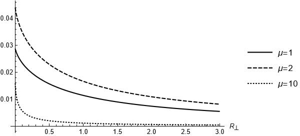
Figure 4: Mixed-sector energy $E_{Qq}$ at coincident points as a function of $\mu$ for various $m$.

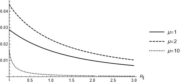
Figure 5: Mixed-sector energy $E_{Qq}$ at coincident points as a function of $m$ for various $\mu$.

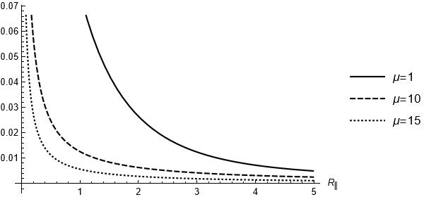
Figure 6: $E_{Qq}$ as a function of $R_\perp$ for $R_\parallel=0$ and various $\mu$.

Figure 7: $E_{Qq}$ as a function of $R_\parallel$ for $R_\perp=0$ and various $\mu$.

• Topological sources: The model supports the analysis of interactions between topological sources (e.g., Dirac points or planar dipoles) in the CS sector. The resulting energies are anisotropic and can generate torques, with the interaction structure controlled by $m$ and $\mu$.

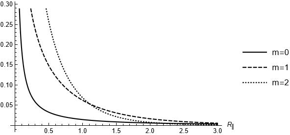
  Figure 8: Interaction energy between two time-like topological sources as a function of $R_\parallel$ for various $m$.

  

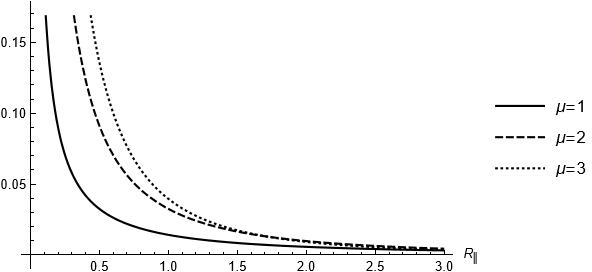
  Figure 9: Interaction energy between two time-like topological sources as a function of $R_\parallel$ for various $\mu$ in the massless case.

  

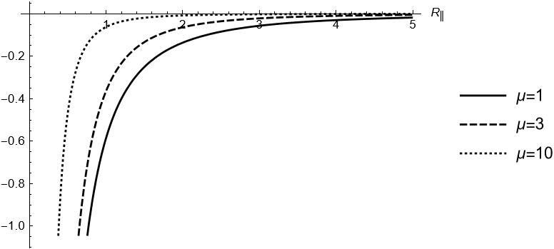
  Figure 10: Interaction energy between two space-like topological sources as a function of $R_\parallel$ for various $\mu$.

  

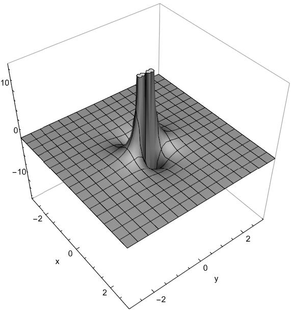
  Figure 11: Torque component for two orthogonal topological sources as a function of position, illustrating the anisotropic response.

Field Solutions and Magnetoelectric Effects

The classical field solutions for both the Maxwell and CS sectors in the presence of a stationary point charge are derived. The Maxwell electric field is the sum of the standard Coulomb field and a correction term dependent on $m$ and $\mu$, which vanishes in the decoupling limit and reproduces the image charge result in the strong coupling limit. The Maxwell magnetic field, which is zero for a static charge in standard electrodynamics, becomes nonzero due to the magnetoelectric coupling, but vanishes for $m=0$ or in the strong coupling regime.

The CS sector fields are also nontrivial: a stationary point charge induces both electric and magnetic fields in the planar sector, with their magnitudes controlled by $m$ and $\mu$. The magnetoelectric effect is thus manifest in both sectors, and is tunable via the model parameters.

Theoretical and Practical Implications

The two-gauge field model provides a flexible and physically motivated framework for simulating magnetoelectric boundaries, with two independent parameters ($m$, $\mu$) allowing for the emulation of a wide range of material responses. The exact propagator enables the calculation of interaction energies, forces, and field configurations for arbitrary source distributions, including the effects of lattice defects and topological excitations.

The model recovers known results in appropriate limits (e.g., perfect conductor, decoupled fields, pure CS theory) and regularizes short-distance divergences in mixed-sector interactions. The ability to describe both surface and near-surface phenomena in a unified field-theoretic language is particularly relevant for the study of topological insulators, quantum Hall systems, and engineered metamaterials.

Potential extensions include the analysis of wave propagation, Casimir effects, and the computation of effective actions for the Maxwell field in the presence of the CS-coupled boundary. The formalism is also amenable to generalization to multiple layers, curved surfaces, and higher-derivative or non-Abelian gauge structures.

Conclusion

The two-gauge field model for magnetoelectric boundaries developed in this work offers a comprehensive and analytically tractable approach to modeling planar material layers with tunable electromagnetic properties. The exact propagator, explicit interaction energies, and field solutions provide a robust foundation for both theoretical investigations and practical applications in condensed matter and materials physics. The model's flexibility and generality suggest its utility in the study of a broad class of boundary phenomena, and its extension to more complex geometries and interactions remains a promising direction for future research.