Equilibrium flow: From Snapshots to Dynamics
Abstract: Scientific data, from cellular snapshots in biology to celestial distributions in cosmology, often consists of static patterns from underlying dynamical systems. These snapshots, while lacking temporal ordering, implicitly encode the processes that preserve them. This work investigates how strongly such a distribution constrains its underlying dynamics and how to recover them. We introduce the Equilibrium flow method, a framework that learns continuous dynamics that preserve a given pattern distribution. Our method successfully identifies plausible dynamics for 2-D systems and recovers the signature chaotic behavior of the Lorenz attractor. For high-dimensional Turing patterns from the Gray-Scott model, we develop an efficient, training-free variant that achieves high fidelity to the ground truth, validated both quantitatively and qualitatively. Our analysis reveals the solution space is constrained not only by the data but also by the learning model's inductive biases. This capability extends beyond recovering known systems, enabling a new paradigm of inverse design for Artificial Life. By specifying a target pattern distribution, we can discover the local interaction rules that preserve it, leading to the spontaneous emergence of complex behaviors, such as life-like flocking, attraction, and repulsion patterns, from simple, user-defined snapshots.

Paper Prompts
Sign up for free to create and run prompts on this paper using GPT-5.
Top Community Prompts
Explain it Like I'm 14
Equilibrium Flow: Turning Snapshots into Motion
Overview
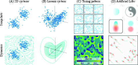
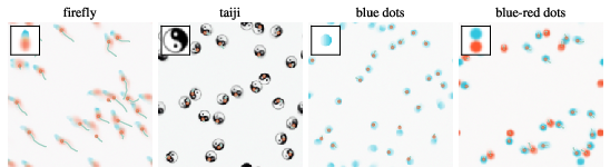
This paper asks a simple but deep question: if all you have are “photos” (snapshots) of a system, can you figure out the hidden rules that make those photos possible? The authors present a method called Equilibrium flow that learns how things move (their dynamics) using only still images of where they tend to be. It works for simple 2D point clouds, famous chaotic systems like the Lorenz attractor, and complex image-like patterns called Turing patterns. It can also be used creatively to “design” artificial life-like behaviors from a picture you choose.
What questions did the authors ask?
- If we only see where things usually are (a distribution of snapshots), how many different sets of rules could keep that pattern stable?
- Can we recover rules that are close to the real ones that generated the data, even if we don’t know the time order of the snapshots?
- Can we use this to invent new rule sets that produce desired patterns and behaviors, such as flocking or attraction/repulsion?
How does the method work? (Simple explanation)
Think about a crowd in a park. At any moment, you take a picture that shows where people are. Even if you don’t watch them move, the map of where they usually stand contains clues about how they walk. If the same crowded spots keep reappearing, the way people move must constantly rearrange them without piling up or emptying places too much. Equilibrium flow finds a “wind field” (a set of arrows that say which way to move at each location) that keeps the overall crowd map the same.
Here’s the idea in everyday terms:
- Treat the density of snapshots (how many points/pixels are at each place) like mass or water.
- Look for a flow that moves things around but doesn’t create new mass or remove it. In math, this is a conservation rule (no net inflow or outflow where it shouldn’t be).
- The key condition the authors enforce is:
- “Don’t squeeze or stretch the density too much” + “Flow should respect the shape of the density.” In compact form: make the quantity “divergence of the flow + alignment with the density’s steepest direction” equal to zero:
- Intuition: is the flow; points “uphill” toward denser regions (like a hill on a map), and measures local spreading/squeezing of the flow. Setting their combination to zero means the flow rearranges things but keeps the overall pattern intact.
- How do we get (the direction toward denser areas)? They use a diffusion model (a modern AI model) that learns to tell which way density increases, even when the true formula for is unknown.
- Computing “divergence” exactly is expensive in high dimensions, so they use a smart shortcut (Hutchinson’s estimator). Imagine checking spread in a few random directions instead of all directions; average those checks to estimate the total spread.
- They train a neural network that outputs the flow field so that the conservation rule above is satisfied at many sample points. They also keep the overall “mean push” zero so the system doesn’t drift away.
A fast, training-free version for big patterns (like images):
- In very high dimensions (e.g., 128×128 images), second-order derivatives are too costly. So they use a neat trick:
- Make a flow that is always perpendicular to the uphill direction. Think of walking along the contour lines on a hiking map (same altitude), not up or down; this naturally preserves the pattern density. Mathematically, use a skew-symmetric matrix to rotate the “uphill” vector by 90 degrees: with .
- To prevent drift and keep things on the data manifold, add a small gentle pull toward denser regions plus a tiny random jiggle (this is a standard “Langevin” term):
- Intuition: flow along the contours (sideways), plus a light nudge uphill, plus slight noise to stabilize and explore.
- For images with two channels, is implemented as a tiny 1×1 convolution that swaps channels with a sign flip (a 90° turn in a 2D plane) — fast and stable.
What did they find?
Across several tests, the method recovers believable, often strikingly good dynamics:
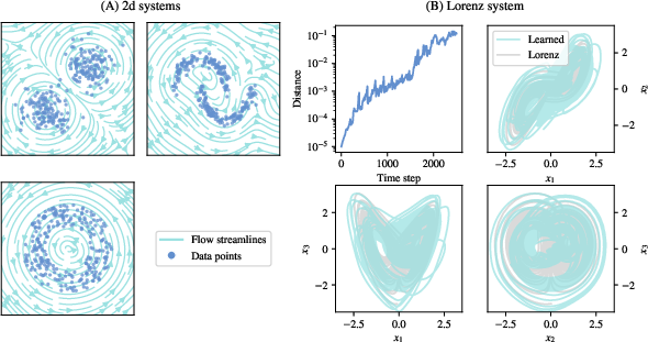
- Simple 2D point clouds:
- Rings lead to rotational flows (things move around the ring but the ring stays a ring).
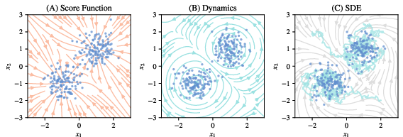
- Two blobs lead to two counter-rotating swirls that keep the overall shape.
- More complex shapes (like “two moons”) produce flows that trace the shape boundary.
- Chaotic Lorenz attractor:
- Even without time labels, the learned flow produces chaotic behavior (small differences grow fast) and preserves the famous butterfly-shaped pattern.
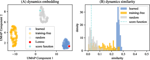
- Multiple training runs produce very similar flows that sit close to the true Lorenz dynamics in a feature comparison, showing both consistency (uniqueness) and decent similarity (fidelity).
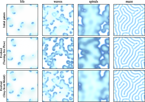
- High-dimensional Turing patterns (Gray–Scott model: spots, spirals, waves, mazes):
- The training-free version recreates the key behaviors: moving “life-like” blobs (solitons), traveling waves and spirals, and static maze-like patterns.
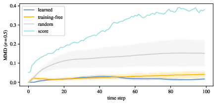
- Quantitatively, the recovered rules are more similar to the correct ones than random alternatives, confirming the patterns carry strong clues about the dynamics.
- Inverse design of artificial life:
- Give the method a target pattern (even a hand-drawn shape). It learns local rules that preserve that pattern distribution.
- When you drop multiple copies into a scene, natural-looking behaviors emerge: flocking, attraction/repulsion, smooth or slow movement depending on the shape’s symmetry.
- Uniqueness and the role of inductive bias:
- When they train neural networks to find the flow, repeated runs converge to almost the same answer (high self-similarity) and are near the ground truth.
- The training-free method explores a broader set of valid flows (more variety), likely because it lacks the neural network’s built-in preference for smooth, simple functions. This shows that both the data and the model’s built-in biases together narrow the solution space.
Why does this matter?
- Science often has “snapshots without timestamps” (cells in a tissue, stars in galaxies, fossils in layers). This method turns those snapshots into likely motion rules, helping us understand, predict, and possibly control complex systems when movies aren’t available.
- It offers a new way to design systems. Instead of trial-and-error searching for rules that make a desired pattern, you can specify the pattern and “invert” to get rules that sustain it — useful in artificial life, materials design, and beyond.
- It suggests a broader idea: patterns contain a lot of information about processes. With the right biases and tools, we can read that information and recover how things move — not perfectly, but in a constrained, meaningful way.
Takeaway
Equilibrium flow is a general recipe for going from “where things are” to “how they move,” using only static data. It works on simple clouds, chaotic systems, and complex image patterns, and even lets you invent new rule sets that create life-like emergent behaviors from a picture you choose. This bridges a gap between seeing patterns and understanding the processes that shape them, opening doors for discovery and design across science and engineering.
Knowledge Gaps
Knowledge gaps, limitations, and open questions
Below is a concise list of what remains missing, uncertain, or unexplored in the paper, framed to be actionable for future work.
- Theoretical identifiability: no formal characterization of the full solution set to ∇·v + vT∇log p = 0; conditions under which the ground-truth dynamics are recoverable (up to a “gauge”) remain unproven.
- Trivial-solution degeneracy: the objective admits v(x) ≡ 0 as a global minimizer; principled mechanisms to exclude or penalize trivial flows (e.g., kinetic-energy normalization, speed constraints, conservation constraints) are not specified or analyzed.
- Exact invariance guarantees: with approximate scores from diffusion models and finite k in Hutchinson’s estimator, there is no proof the learned dynamics preserve p(x) (or pτ) exactly; quantify approximation error and provide convergence guarantees.
- Stationarity assumption: the method assumes an invariant (equilibrium) distribution; extensions to slowly drifting or non-stationary distributions (quasi-stationary regimes) are not developed.
- Role of inductive bias vs. data: while inductive biases are hypothesized to constrain solutions, there is no quantitative theory relating data manifold properties (sparsity, topology, symmetries) and model biases to solution uniqueness.
- Dependence on score quality: sensitivity of learned dynamics to bias/variance in score estimates, model misspecification, and diffusion training regimes (architecture, dataset size) is not quantified.
- Choice of noise level τ: actionable criteria or data-driven procedures for selecting τ (balancing smoothing vs. fidelity) are not provided; impacts on solution space and stability are unstudied.
- Divergence estimation: computationally heavy Hutchinson-based divergence limits scalability; alternatives (e.g., divergence-free parameterizations, spectral/Green’s function estimators, learned Jacobian–vector products with low-rank structure) are not explored.
- Boundary conditions: handling of domain boundaries (periodic, reflective, absorbing) is unspecified; how boundary choices alter learned dynamics and invariance is unaddressed.
- Existence/uniqueness of ODE solutions: no constraints imposed on v (e.g., Lipschitz constants) to guarantee well-posedness and numerical stability of flows over long horizons.
- Stochastic dynamics invariance: the irreversible Langevin SDE (with approximate scores) lacks guarantees of stationarity/ergodicity for the target distribution; quantify invariant-measure deviation and mixing rates.
- Training-free expressivity: the skew-symmetric 1×1 convolution used for high-dimensional patterns is severely restricted; the need for spatially varying/non-local skew operators (larger receptive fields, kernels with structure) is not assessed.
- Sign/rotation ambiguity in training-free solutions: γ is selected using ground truth; an unsupervised criterion to resolve directionality (e.g., by maximizing self-consistency or propagation metrics) is missing.
- Partial observability: the approach assumes full-state snapshots; extensions to latent-variable systems or partial observations (e.g., learning dynamics on observed marginals consistent with hidden variables) are not considered.
- Sample complexity: no analysis of how many snapshots are needed (vs. dimensionality and manifold complexity) to reliably constrain dynamics or train diffusion models with adequate score accuracy.
- Robustness to data noise and sampling bias: sensitivity to measurement noise, outliers, covariate shift, and non-representative snapshot sampling is not evaluated; no uncertainty quantification over learned dynamics.
- Evaluation breadth for chaotic systems: beyond positive Lyapunov exponents, richer metrics (Lyapunov spectrum, correlation/fractal dimension, invariant-measure distances, return-time statistics) are not reported.
- Metrics for high-dimensional patterns: fidelity for Turing patterns is mainly qualitative or based on short-horizon cosine differences; morphology-aware metrics (power spectra, structure tensors, topological summaries via persistent homology) and long-horizon stability tests are lacking.
- Generalization and OOD behavior: how learned dynamics behave off the data manifold or under previously unseen pattern regimes is not studied; failure modes and guardrails are unspecified.
- One-stage training: the two-stage pipeline (score then dynamics) is not compared to end-to-end formulations that might reduce error compounding and cost; tractable joint objectives are an open direction.
- Inductive-bias design: systematic ways to impose beneficial biases (e.g., symmetry, locality, conservation laws, sparsity in vector potentials) for both trained and training-free variants are not developed.
- Physical constraints and interpretability: methods to enforce known physics (e.g., energy, momentum, symmetry groups) or recover interpretable rule sets (e.g., PDE terms, local interaction kernels) are not provided.
- Numerical stability and integration choices: effects of integrators, step sizes, stiffness, and discretization errors on long-term behavior and invariance are not assessed.
- Multi-modal and low-density regions: behavior of learned flows near low-density “gaps” (e.g., tunneling across modes, spurious drift) is not characterized; regularization to respect mode separation is absent.
- Non-Euclidean domains: extensions to manifolds, graphs, or categorical state spaces (where divergence and scores have different geometry) are not addressed.
- Reproducibility and ablations: key hyperparameters (k for Hutchinson, batch norm design, learning rates, network width/depth) and their effects on convergence, uniqueness, and fidelity lack systematic ablation.
- Inverse design control: for Artificial Life, controllability of speed, interaction range, collision avoidance, and multi-agent coordination is not parameterized; quantitative evaluation of emergent behaviors is missing.
- Selecting among multiple valid dynamics: criteria to choose “minimal,” “simplest,” or “most physical” dynamics from the admissible set (e.g., complexity regularizers, action minimization, entropy production) are not defined.
Practical Applications
Overview
From the paper “Equilibrium flow: From Snapshots to Dynamics,” the central innovation is a framework that infers continuous-time dynamics directly from static (unordered) data distributions by enforcing a local conservation constraint using the score of the distribution (estimated via diffusion models). It includes:
- A learnable vector-field approach (with Hutchinson’s trace estimator) that scales to low/mid dimensions and recovers qualitative properties (e.g., chaos in Lorenz).
- A training-free, high-dimensional variant that constructs valid dynamics via a skew-symmetric transform of the score, stabilized by an irreversible Langevin term—effective for image-like pattern data (e.g., Gray-Scott Turing patterns).
- An inverse-design paradigm for Artificial Life: users specify pattern distributions and the method discovers local interaction rules that preserve them, yielding emergent behaviors.
Below are actionable applications, grouped by deployment horizon, with sector links, potential tools/workflows, and feasibility caveats.
Immediate Applications
- Software/ML and Computer Graphics
- Pattern-preserving animation and simulation from static datasets
- Use case: Turn textures, logos, or scientific images into physically plausible, endless motion loops or interactive simulations that preserve the original style/distribution.
- Workflow: Train a diffusion model to estimate the score on snapshots → fit Equilibrium flow (learned or training-free) → generate motion consistent with the distribution → evaluate via invariance loss and stability metrics.
- Tools/products: “Pattern-to-Dynamics” plugin for Diffusers; “EquilibriumFlow” module; real-time “SkewConv + Langevin” layer for image dynamics; UMAP-based diagnostics for uniqueness/fidelity.
- Assumptions/dependencies: Stationarity (snapshot distribution approximates an invariant measure), good score estimation, sufficient coverage of the data manifold, manageable dimensionality or use of the training-free variant.
- Robotics (swarms, formation control)
- Inverse design of local interaction rules from target formations/patterns
- Use case: Derive decentralized policies for drone/robot swarms that maintain/track a desired spatial pattern (flocking, coverage, rotating rings).
- Workflow: Specify target pattern distribution (shape library, hand-drawn templates) → learn training-free dynamics via skew-symmetric transforms of the score → synthesize controllers (local rules) → validate in multi-agent simulation.
- Tools/products: “ALife Designer” for pattern-to-policy; on-robot inference via 1×1 SkewConv; sim-to-real adapters.
- Assumptions/dependencies: Patterns must map to observable state variables; local sensing/communication; safety constraints; stationarity of the target distribution in the operational environment.
- Synthetic Biology / Artificial Life (in silico)
- Rapid prototyping of emergent behaviors from desired morphologies
- Use case: Discover local update rules that preserve user-specified patterns (e.g., “firefly” flocking), to study form–function relationships and emergent dynamics.
- Workflow: Build a dataset by scattering/rotating a target motif → apply training-free dynamics (skew-symmetric score transform + Langevin) → screen behaviors (flocking, attraction/repulsion).
- Tools/products: Interactive ALife sandboxes; pattern-conditioned rule generators; behavior analytics toolkit (trajectory statistics, Lyapunov measures).
- Assumptions/dependencies: Digital-only for now; mapping from pixel/state to physical biochemistry is nontrivial; interpretability of local rules may be limited.
- Materials/Manufacturing QA and Monitoring
- Stationary-pattern change detection via distribution-preserving dynamics
- Use case: Learn equilibrium flows on stable microstructure or wafer-map patterns; flag deviations when new snapshots violate learned invariance (drift/anomaly detection).
- Workflow: Train score and learn dynamics on “healthy” snapshot distributions → monitor divergence/consistency over time → raise alerts.
- Tools/products: “PatternGuard” for stationarity testing; real-time dashboards.
- Assumptions/dependencies: Data represent a stationary process; domain shifts are detectable through invariance violations; consistent imaging conditions.
- Education and Scientific Communication
- Interactive demos for chaos, Helmholtz decomposition, pattern formation
- Use case: Reconstruct Lorenz-like flows from point clouds; draw a pattern and watch emergent motion that preserves it; build intuition about score-based models and conservation laws.
- Workflow: Notebooks/apps that train a small score model on toy data → learn flows → visualize dynamics; inspect Lyapunov exponents and cosine similarity to ground truth.
- Tools/products: Classroom-ready notebooks; web demos; curriculum modules.
- Assumptions/dependencies: Small compute; clear didactic examples.
- Vision/Data Augmentation
- Style-preserving motion augmentation
- Use case: Augment datasets with realistic motion that preserves class/style distributions for robustness testing or synthetic video generation.
- Workflow: Fit score on images → derive dynamics → simulate short trajectories as motion-augmented samples; keep class distribution intact.
- Tools/products: “Equilibrium Augment” pipeline.
- Assumptions/dependencies: Stationary class/style distributions; careful validation to avoid distribution drift.
- Environmental Visualization (non-predictive)
- Realistic flow visualization along density isocontours
- Use case: Generate compelling animations of plankton/bloom distributions or terrain/vegetation patterns without forecasting claims.
- Workflow: Estimate score on satellite imagery patches → training-free dynamics to produce flows along equal-density surfaces → visualization overlays.
- Tools/products: Visualization plugins for GIS tools.
- Assumptions/dependencies: Strictly for visualization; stationarity and observational mapping must be acknowledged to avoid misuse as forecasts.
Long-Term Applications
- Life Sciences: Systems and Developmental Biology
- Inferring interaction rules or coarse-grained dynamics from snapshot omics/imaging
- Use case: From tissue/cell snapshots (e.g., histology, live-cell imaging), infer plausible, distribution-preserving flows to hypothesize underlying signaling/cell–cell interaction rules; explore morphogenesis from static patterns.
- Potential products: Hypothesis generation platforms; virtual perturbation tools that conserve observed distributions; experimental design assistants.
- Dependencies: Stationarity or quasi-steady-state assumptions; partial observability; mapping from pixels to latent biological states; validated score models for noisy bio data; ethical use and experimental corroboration.
- Cosmology and Astrophysics
- Constraining plausible dynamics from spatial distributions
- Use case: Use galaxy/stellar distributions to constrain families of distribution-preserving flows; test qualitative consistency with known physics; explore model spaces efficiently.
- Products/workflows: Score estimators for astronomical catalogs; flow-based model comparison; UMAP/fidelity diagnostics.
- Dependencies: Selection effects, survey bias corrections, coarse-graining; whether stationarity assumptions hold; linking learned flows to physically interpretable fields.
- Climate and Geophysical Sciences
- Snapshot-based closures and subgrid modeling
- Use case: From ensembles of stationary snapshot fields (e.g., turbulent patches), infer distribution-preserving dynamics for use as closures or surrogate simulators.
- Products/workflows: Hybrid PDE–ML surrogates with Equilibrium flow components; stability-informed parameterizations.
- Dependencies: Physical constraints (energy/casuality), boundary conditions, nonstationarity of climate signals, rigorous validation.
- Materials Design and Process Engineering
- Inverse design of reaction–diffusion microstructures
- Use case: Specify a target microstructure distribution; discover local rules/parameters that preserve it; use as starting points for lab calibration (e.g., feed/kill rates in Gray-Scott–like systems).
- Products/workflows: “Pattern-to-Process” inverse-design tools that propose process windows; integration with lab robotics for closed-loop optimization.
- Dependencies: Mapping from learned local rules to actionable process parameters; experimental uncertainty; multi-physics coupling.
- Healthcare and Digital Pathology
- Tumor microenvironment and tissue remodeling hypotheses
- Use case: From cross-sectional histopathology images, formulate candidate distribution-preserving flows that reflect cell migration/ECM remodeling dynamics; probe intervention “what-ifs” digitally.
- Products/workflows: Decision support for hypothesis generation; virtual tissue sandboxes.
- Dependencies: Strong stationarity violations in disease progression; confounders (staining, sampling); clinical validation; regulatory considerations.
- Finance and Economics
- Cross-sectional state flow modeling under stationarity
- Use case: From distributions of market states or agent configurations, infer neutral (distribution-preserving) flows for stress testing, scenario design, or agent-based calibration.
- Products/workflows: Market microstructure sandboxes; cross-sectional simulators.
- Dependencies: Market nonstationarity; mapping from observed vectors to well-defined state space; governance and risk management.
- Energy, Mobility, and Smart Cities
- Decentralized control from target spatial distributions
- Use case: Derive local rules that maintain desired traffic/energy load patterns (e.g., peak-shaving distributions, coverage densities).
- Products/workflows: Controller synthesis tools for multi-agent infrastructure (EV fleets, micromobility swarms).
- Dependencies: Real-time constraints, safety, heterogeneity, sensing; regulatory approvals.
- Safety, Governance, and Policy
- Monitoring stationarity and drift; misuse mitigation
- Use case: Institutions adopt “Equilibrium flow” monitors to detect undesirable distribution shifts in critical systems; develop guidance for responsible deployment of generative dynamics that look realistic but are not forecasts.
- Products/workflows: Compliance checks using invariance metrics; documentation of assumptions; audit trails for data and model bias.
- Dependencies: Domain-specific definitions of stationarity; interpretability; standards for disclosure to prevent misinterpretation.
Cross-cutting Assumptions and Dependencies
- Data and distributional assumptions
- Snapshots are i.i.d. from (approximately) a stationary/invariant distribution; adequate sample coverage, quality, and consistent measurement.
- Modeling assumptions
- Underlying dynamics are well-approximated by continuous-time ODE/SDE fields; the score function of the data distribution exists and is learnable.
- Estimation and compute
- Reliable score estimation via diffusion models; choice of noise level τ impacts stability vs fidelity; Hutchinson’s estimator scales poorly in very high dimensions (favor training-free approach).
- Identifiability and inductive bias
- Multiple dynamics can preserve a distribution; neural architectures inject helpful biases (smoothness, locality) that constrain solutions; interpretability may be limited without domain constraints.
- Physical and domain constraints
- For scientific use, incorporate conservation laws, boundary conditions, symmetries; validate with domain metrics (e.g., Lyapunov exponents, conserved quantities).
- Risk and governance
- Avoid presenting generated dynamics as precise forecasts; disclose assumptions; ensure safety when deploying local rules to physical systems.
These applications leverage the paper’s main insight: static distributions constrain plausible dynamics far more than naive intuition suggests—especially when combined with principled inductive biases—making it possible to infer, design, and monitor complex systems from snapshots alone.
Glossary
- Artificial Life: A research field exploring life-like behaviors and systems in computational or synthetic media. "enabling a new paradigm of inverse design for Artificial Life."
- Batch normalization: A neural network technique that normalizes layer outputs to stabilize and speed up training. "we apply a batch normalization layer to the output of the neural network~, forcing it to be zero-mean over each mini-batch."
- Continuity equation: A conservation law expressing that probability (or mass) is locally conserved under a flow. "this approach leads us to the continuity equation:"
- Cosine similarity: A measure of similarity between two vectors based on the cosine of the angle between them. "Cosine similarity to the ground-truth Lorenz dynamics."
- Curl: A measure of a vector field’s local rotation; non-zero curl indicates rotational components in dynamics. "this inevitably misses a significant portion of dynamics that have curl."
- Diffusion model: A generative model that learns data distributions by denoising progressively noised data. "a quantity that can be effectively estimated with pre-trained diffusion models"
- Divergence-free: Describes a vector field with zero divergence, indicating incompressible flow. "a valid, divergence-free vector field"
- Fokker-Planck-Kolmogorov equation: A partial differential equation governing the time evolution of probability densities under stochastic dynamics. "The Fokker-Planck-Kolmogorov equation is typically used to model the time evolution of distributions"
- Gray-Scott model: A reaction-diffusion system that generates complex spatial patterns via two interacting chemical species. "For high-dimensional Turing patterns from the Gray-Scott model, we develop an efficient, training-free variant"
- Helmholtz decomposition: The representation of a vector field as the sum of a curl-free (gradient) part and a divergence-free (solenoidal) part. "From the perspective of Helmholtz decomposition, any vector field can be decomposed into a curl-free (gradient) part and a divergence-free (curl) part."
- Hutchinson's Trace Estimator: A stochastic method to estimate the trace (and thus divergence) of a Jacobian without explicit computation. "We can, however, efficiently approximate it using Hutchinson's Trace Estimator~\citep{hutchinson1989stochastic}:"
- Inductive bias: The set of assumptions a learning algorithm uses to generalize beyond the observed data. "our analysis reveals the solution space is constrained not only by the data but also by the learning model's inductive biases."
- Irreversible Langevin SDE: A stochastic differential equation with non-reversible drift that preserves a target distribution while enhancing mixing. "This yields an irreversible Langevin SDE~\citep{Hwang_2005, rey2015irreversible}:"
- Kolmogorov complexity: The length of the shortest program that can generate a given object; a measure of algorithmic complexity. "Kolmogorov complexity renders a direct search for such minimal dynamics for patterns uncomputable"
- Lorenz attractor: A strange attractor arising from the Lorenz system, exhibiting chaotic behavior. "recovers the signature chaotic behavior of the Lorenz attractor."
- Lorenz system: A classic set of three ODEs that exhibit deterministic chaos. "the recovered dynamics of the chaotic Lorenz system."
- Lyapunov exponent: A quantity characterizing the average exponential divergence or convergence of nearby trajectories; positive values indicate chaos. "indicating a positive Lyapunov exponent."
- Maximum mean discrepancy (MMD): A kernel-based statistical distance between distributions used for model fitting and two-sample testing. "fit distributions via maximum mean discrepancy~(MMD)"
- Neural ODEs: Models that parameterize continuous-time dynamics with neural networks and are trained via ODE solvers. "rely on computationally expensive neural ODEs to model dynamics"
- Normalization flows: Invertible neural transformations that map simple base distributions to complex ones with tractable likelihoods. "or normalization flows."
- Positional encoding: A technique to inject high-frequency basis functions into inputs, enabling networks to represent fine variations. "we incorporate positional encoding:"
- Reaction-diffusion equations: PDEs modeling the interplay between local reactions and spatial diffusion that produce patterns. "through a system of reaction-diffusion equations:"
- Score function: The gradient of the log-density, pointing toward higher probability regions of a distribution. "directly uses the score function of a density distribution as the force field"
- SiLU: The Sigmoid Linear Unit activation function, also known as Swish, used to improve training dynamics. "we use SiLU~\citep{ramachandran2017swish, elfwing2018sigmoid} instead of ReLU."
- Skew-symmetric matrix: A matrix A satisfying A⊤ = −A, generating divergence-free linear flows when applied to vectors. "is a skew-symmetric matrix (i.e.,~)."
- Stein identity: An identity relating expectations under a distribution to expectations involving its score function, used in inference and learning. "While the well-known Stein identity~\citep{liu2016kernelized} requires this term to be zero only in expectation,"
- Turing patterns: Spatial patterns arising from reaction-diffusion systems as predicted by Turing’s theory of morphogenesis. "By applying our method to Turing patterns, we can recover dynamics that preserve both qualitative and quantitative features of the ground truth."
- UMAP: A nonlinear dimension reduction technique preserving local and global structure in embeddings. "We first visualize the space of solutions by applying the UMAP dimension reduction method~\citep{umap} to the representations"
- U-Net: A convolutional neural network architecture with encoder-decoder and skip connections, common in image-to-image tasks. "We adopt a minimal 2D U-Net, based on the diffusers library's UNet2DModel"
- Vector-Jacobian products: Efficient computations of Jacobian-vector multiplications used in autodiff for higher-order derivatives. "our gradient descent process involves vector-Jacobian products that require non-zero second-order gradients"
- Wiener process: A continuous-time stochastic process with independent Gaussian increments; the mathematical model for Brownian motion. "where~ is the Wiener process."
Collections
Sign up for free to add this paper to one or more collections.