Learning Under Laws: A Constraint-Projected Neural PDE Solver that Eliminates Hallucinations

Abstract: Neural networks can approximate solutions to partial differential equations, but they often break the very laws they are meant to model-creating mass from nowhere, drifting shocks, or violating conservation and entropy. We address this by training within the laws of physics rather than beside them. Our framework, called Constraint-Projected Learning (CPL), keeps every update physically admissible by projecting network outputs onto the intersection of constraint sets defined by conservation, Rankine-Hugoniot balance, entropy, and positivity. The projection is differentiable and adds only about 10% computational overhead, making it fully compatible with back-propagation. We further stabilize training with total-variation damping (TVD) to suppress small oscillations and a rollout curriculum that enforces consistency over long prediction horizons. Together, these mechanisms eliminate both hard and soft violations: conservation holds at machine precision, total-variation growth vanishes, and entropy and error remain bounded. On Burgers and Euler systems, CPL produces stable, physically lawful solutions without loss of accuracy. Instead of hoping neural solvers will respect physics, CPL makes that behavior an intrinsic property of the learning process.

• The paper introduces Constraint-Projected Learning (CPL), a framework that projects neural network outputs onto constraint sets to enforce conservation, entropy, and shock conditions.
• It employs differentiable projection operators that integrate seamlessly with backpropagation, achieving near-zero violations as validated on Burgers’ equation with minimal performance overhead.
• Combining Total-Variation Damping (TVD) with a rollout curriculum, the method stabilizes long-horizon predictions, ensuring physically consistent and accurate neural PDE solutions.

Constraint-Projected Neural PDE Solvers: Eliminating Hallucinations via Law-Constrained Optimization

Introduction

The paper introduces Constraint-Projected Learning (CPL), a framework for training neural PDE solvers that strictly enforces physical laws at every update, thereby eliminating both hard and soft hallucinations. Hallucinations in neural solvers manifest as violations of conservation, entropy, or admissibility, leading to physically implausible predictions even when statistical accuracy is high. CPL addresses this by projecting network outputs onto the intersection of constraint sets defined by conservation, Rankine–Hugoniot (RH) balance, entropy, and positivity, ensuring that every prediction is physically admissible. The projection is differentiable and computationally efficient, adding only ~10% overhead, and is compatible with standard backpropagation.

Geometric Formulation of Law-Constrained Learning

CPL reframes the optimization landscape by restricting updates to the lawful manifold $\mathcal{C}$, defined as the intersection of all constraint sets. The update rule is:

$$\theta_{k+1} = \Pi_{\mathcal{C}}\left(\theta_k - \eta \nabla_\theta L\right)$$

where $\Pi_{\mathcal{C}}$ is the projection operator. This geometric approach ensures non-expansiveness and stability, as projections onto convex (or locally convex) sets cannot amplify errors. Each constraint—finite-volume conservation, RH balance, entropy admissibility, positivity, and divergence-free structure—is implemented as a differentiable projector, allowing seamless integration with gradient-based learning.

Discretization: From Differential Laws to Finite Constraints

Physical laws are translated from strong (differential) form to weak (integral) form, enabling enforcement over finite regions rather than pointwise. The domain is discretized into control volumes, and conservation is enforced via finite-volume residuals:

$$\mathcal{R}_i^n = \frac{\bar{\mathbf{U}}_i^{n+1} - \bar{\mathbf{U}}_i^n}{\Delta t} + \frac{1}{|C_i|} \sum_{f \in \partial C_i} |f|\,\Phi_{i,f}^n - \bar{\mathbf{S}}_i^n$$

where $\Phi_{i,f}^n$ is the numerical flux. Local conservation implies global conservation due to the telescoping property of fluxes.

Shock and Entropy Constraints

Rankine–Hugoniot Condition

Shocks are enforced via the RH jump condition:

$$\llbracket \mathbf{F}(\mathbf{U}) \cdot \mathbf{n} \rrbracket = s_n \llbracket \mathbf{U} \rrbracket$$

This is implemented as a penalty on the mismatch at detected shock interfaces, ensuring correct propagation and steepness of discontinuities.

Entropy Admissibility

The entropy constraint selects the physically valid weak solution:

$$\partial_t \eta(\mathbf{U}) + \nabla \cdot \mathbf{q}(\mathbf{U}) \leq 0$$

Discretized as a cell-wise penalty on positive entropy residuals, this ensures thermodynamic consistency.

Stability Constraints: Positivity and Total-Variation Damping

Positivity is enforced via clamping or softplus transformations, preventing negative densities or pressures. Total-Variation Damping (TVD) penalizes increases in spatial roughness:

$$L_{\mathrm{TVD}} = \left\langle \max\left(0, TV(U^{n+1}) - TV(U^n)\right) \right\rangle$$

This suppresses non-physical oscillations without blurring genuine shocks.

Divergence-Free Projection

For incompressible or magnetically balanced systems, the Helmholtz projection ensures divergence-free fields:

$$\mathbf{v}_\perp = \mathbb{P}\,\mathbf{v}, \quad \mathbb{P} = I - \nabla \Delta^{-1} \nabla \cdot$$

This is implemented via FFT or multigrid solvers and is 1-Lipschitz, preserving stability.

Implementation: Training Loop and Diagnostics

The training loop integrates all constraints:

1. Forward pass: $\mathbf{U} = \text{net}(x, t)$
2. Compute residuals for conservation, RH, entropy, TVD, and bounds.
3. Assemble total loss with adaptive weights.
4. Gradient update.
5. Sequential projection through all constraint operators.

Reliability is measured via mass/energy drift, entropy violations, shock alignment, TVD growth, and bound violations, summarized in a Physics Violation Score (PVS).

Berger-Limited Reconstruction and Empirical Results

The Berger limiter is used for shock sharpening, selectively steepening discontinuities while maintaining monotonicity and admissibility. On Burgers’ equation ($\nu=0.01$, $N=128$), CPL alone achieves:

• $\text{MSE}_{\text{CPL}} = 1.31 \times 10^{-6}$
• $\text{MAE}_{\text{CPL}} = 4.2 \times 10^{-4}$
• $|\text{Mass drift}| \approx 4.8 \times 10^{-10}$
• $$\langle \mathcal{E}^{\mathrm{RH}} \rangle \approx 4.4 \times 10^{-10}$$

Berger activates in 19% of cells, steepening shocks with negligible impact on conservation or entropy errors.

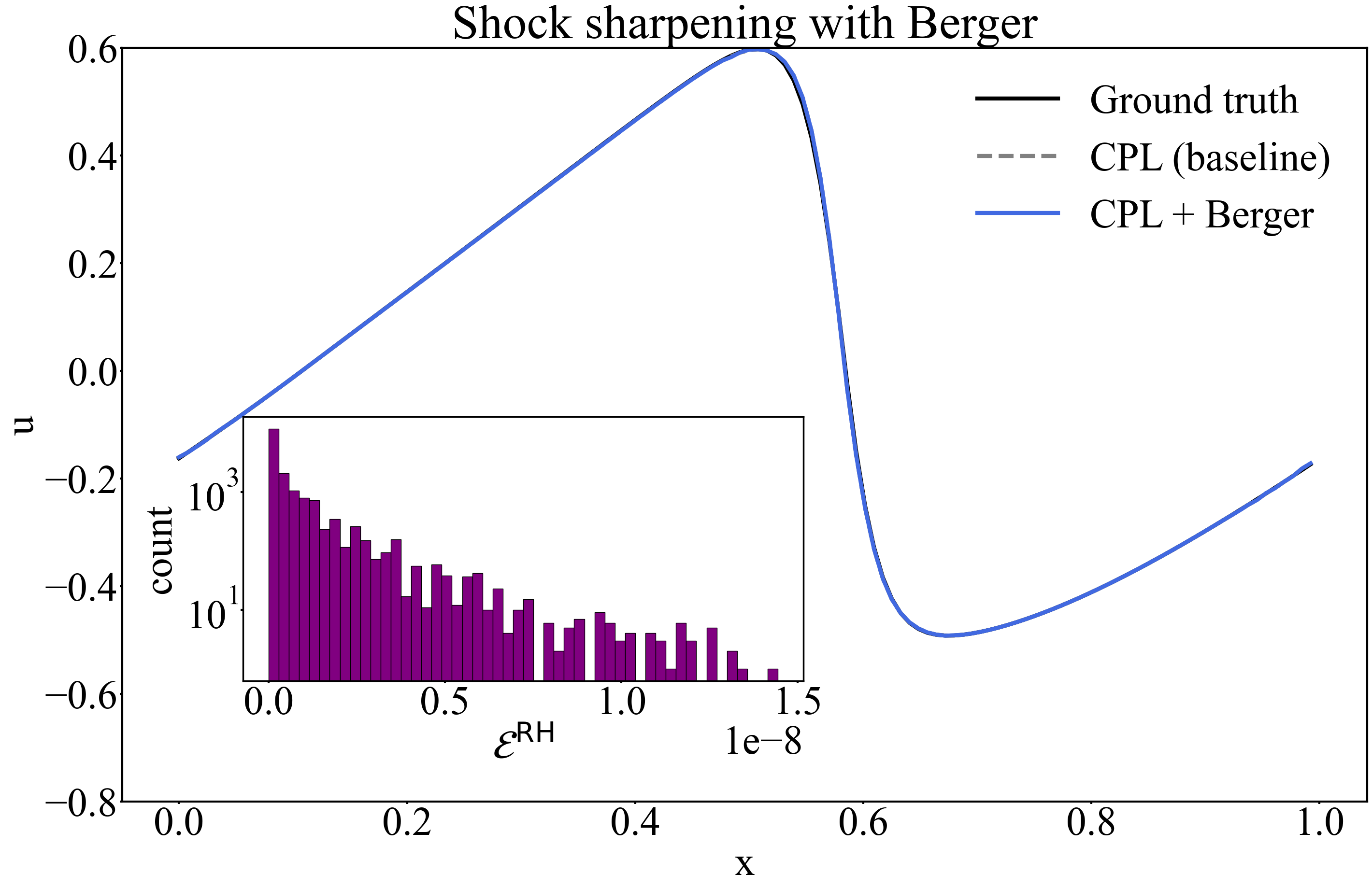
Figure 1: The Berger limiter steepens the shock front, matching the reference solution while conserving fluxes and maintaining entropy admissibility.

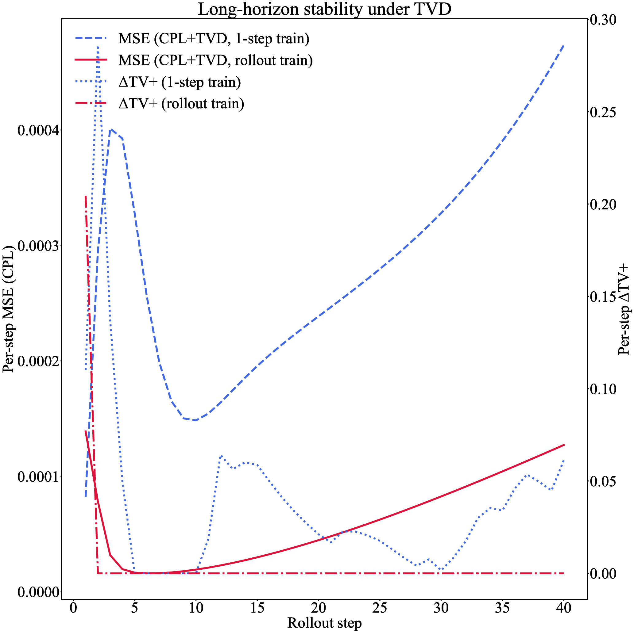
Long-Horizon Stability via TVD and Rollout Curriculum

TVD suppresses the accumulation of small-scale oscillations over long rollouts. Training with a rollout curriculum (increasing prediction steps $R$) further stabilizes the solution:

• One-step CPL+TVD: $\text{MSE}_{\text{CPL}} = 9.7 \times 10^{-7}$, $\langle \Delta TV^+ \rangle = 0.0$
• 40-step rollout: $\text{MSE}_{\text{CPL}} = 2.8 \times 10^{-4}$, mass/RH errors $< 10^{-9}$
• Rollout-trained CPL+TVD: $\text{MSE}_{\text{CPL}} = 6.0 \times 10^{-5}$ after 40 steps, $\langle \Delta TV^+ \rangle = 5.1 \times 10^{-3}$

  Figure 2: TVD and rollout curriculum maintain bounded error and total variation over forty-step rollouts, suppressing lawful drift and oscillatory artifacts.

Quantitative Suppression of Hallucinations

CPL+TVD eliminates hard violations (mass, RH, negative densities) to machine precision and suppresses soft violations (entropy, roughness) to negligible levels. The fraction of cells with positive entropy residuals is $0.23$–$0.31$, with small mean magnitude ($\sim 10^{-3}$–$10^{-2}$). The projection step ensures that raw outputs are immediately corrected, preventing the amplification of deviations.

Universality and Scalability

The CPL mechanism is universal for any constraint expressible as a projection. TVD is agnostic to the underlying PDE. Performance constants depend on the geometry of the constraint sets, but the learning principle is portable across domains. Extension to multi-dimensional Euler, MHD, or reactive flows requires only appropriate projectors (e.g., HLLC fluxes, entropy pairs).

Conclusion

Constraint-Projected Learning, combined with TVD and rollout curriculum, yields neural PDE solvers that are accurate, stable, and physically consistent over long horizons. CPL enforces conservation and admissibility by construction, TVD suppresses non-physical roughness, and rollout training imparts temporal discipline. Empirical results on Burgers’ equation demonstrate near-zero violation of physical laws and bounded error over extended rollouts. The framework is extensible to higher-dimensional and more complex systems, contingent on the availability of differentiable projectors. Future work will focus on efficient projection solvers and adaptive TVD for stiff or multiscale problems.

The approach demonstrates that neural solvers can be trained to respect physical laws indefinitely, transforming scientific machine learning from data-driven regression to law-constrained evolution.