Intermittent time series forecasting: local vs global models

Abstract: Intermittent time series, characterised by the presence of a significant amount of zeros, constitute a large percentage of inventory items in supply chain. Probabilistic forecasts are needed to plan the inventory levels; the predictive distribution should cover non-negative values, have a mass in zero and a long upper tail. Intermittent time series are commonly forecast using local models, which are trained individually on each time series. In the last years global models, which are trained on a large collection of time series, have become popular for time series forecasting. Global models are often based on neural networks. However, they have not yet been exhaustively tested on intermittent time series. We carry out the first study comparing state-of-the-art local (iETS, TweedieGP) and global models (D-Linear, DeepAR, Transformers) on intermittent time series. For neural networks models we consider three different distribution heads suitable for intermittent time series: negative binomial, hurdle-shifted negative binomial and Tweedie. We use, for the first time, the last two distribution heads with neural networks. We perform experiments on five large datasets comprising more than 40'000 real-world time series. Among neural networks D-Linear provides best accuracy; it also consistently outperforms the local models. Moreover, it has also low computational requirements. Transformers-based architectures are instead much more computationally demanding and less accurate. Among the distribution heads, the Tweedie provides the best estimates of the highest quantiles, while the negative binomial offers overall the best performance.

• The paper demonstrates that global approaches, especially D-Linear, outperform local models in forecasting intermittent time series.
• It evaluates various architectures and distribution heads, emphasizing the role of negative binomial and Tweedie outputs for reliable forecasts.
• The study highlights the trade-off between model complexity and computational efficiency, urging simpler methods over deep architectures.

Intermittent Time Series Forecasting: Systematic Comparison of Local and Global Models

Overview and Motivation

Forecasting intermittent time series—characterized by frequent zeros and heavy-tailed positive outcomes—remains a critical challenge in domains such as supply chain and retail inventory management, where accurate probabilistic forecasts underpin strategic and operational decisions. While local models (trained per series) have dominated this domain, especially for count and sparse demand data, recent advances in deep learning have popularized global models trained across multiple time series. However, global architectures' empirical efficacy for intermittent series, particularly regarding distributional forecast quality and computational cost, was hitherto underevaluated.

This paper provides the first comprehensive, large-scale empirical study benchmarking state-of-the-art local and global probabilistic forecasting models on real-world intermittent time series, systematically interrogating the roles of architecture, distributional output heads, and computational efficiency across diverse datasets. Of particular note is the inclusion of advanced distribution heads—the Tweedie and hurdle-shifted negative binomial (HSNB)—with neural architectures for the first time in this context.

Modeling Approaches

Local Models

Three representative local models are evaluated:

• In-sample Quantiles (ISQ): Empirical quantile-based forecasts assuming i.i.d. observations, surprisingly resilient for highly intermittent data.
• iETS: An intermittent extension of exponential smoothing based on Croston's decomposition, forecasting occurrence and size components separately.
• TweedieGP: A Bayesian approach employing a Gaussian Process prior with Tweedie likelihood, enabling rich posterior predictive distributions, particularly advantageous for modeling heavy tails and zero inflation.

Global Models

Global architectures trained on collections of series include:

• Feed-forward Neural Networks (FNNs): Shallow, multi-horizon networks outputting parameters for probabilistic distributions.
• D-Linear: A lightweight, linear model that decomposes input series into trend and remainder with moving averages before applying a linear layer, supporting efficient multi-horizon probabilistic output.
• DeepAR: LSTM-based recurrent networks using autoregressive sampling, historically dominant for global time series density estimation.
• Transformers (Vanilla, Informer, Autoformer): Sequence-to-sequence models leveraging various attention and decomposition mechanisms. These models have recently been popular for general time series, but their suitability for intermittent data is questioned here.

Distribution Heads

Forecast distribution choices are critical for capturing the idiosyncratic distribution of intermittent demand. The paper contrasts:

• Negative Binomial: Supports overdispersion and mass at zero, with unimodal positive support.
• HSNB: An explicit mixture with separate mass at zero and shifted negative binomial for positives—capable of modeling bimodality.
• Tweedie: Continuous, highly flexible for zero-inflation and heavy tails, especially suitable for real-valued intermittent series.

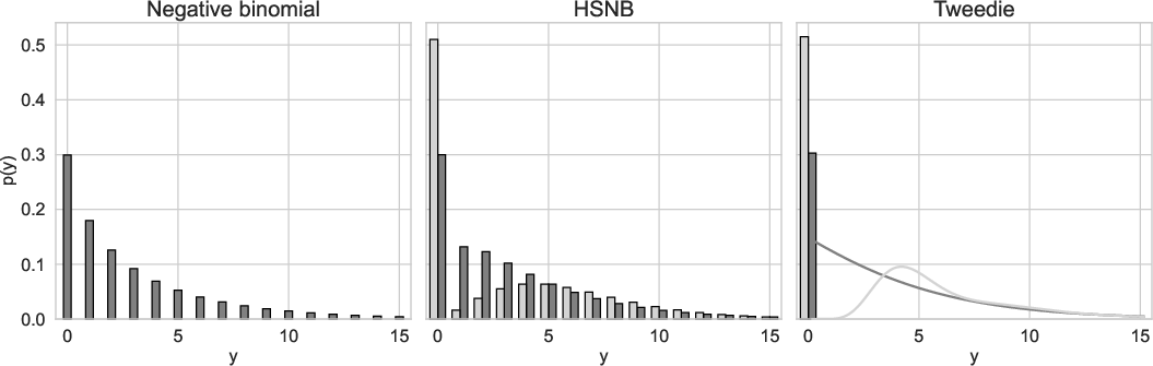
  Figure 1: Each distribution (negative binomial, Tweedie, HSNB) with mean 3 and variance 15, illustrating unique parameterizations, zero mass, and support characteristics.

Experimental Protocol

The evaluation spans five large real-world datasets (M5, UCI, Auto, Carparts, RAF), covering thousands of time series with varying frequencies, lengths, intermittency, and volatility. Models are assessed primarily via scaled quantile loss (multiple upper quantiles) and RMSSE, with careful attention to the stability and reproducibility of results (ten independent runs per configuration).

Computational Efficiency

Resource efficiency is analyzed in the context of both model training and inference. The D-Linear and FNN architectures exhibit significantly reduced computational demands and parameter budgets compared to deep recurrent and transformer models, whose vast parameter counts (up to two orders of magnitude higher) and autoregressive sampling create substantial overhead.

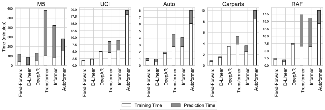
Figure 2: Training and prediction times (minutes) for neural architectures; transformer models require orders of magnitude more runtime than shallow methods.

Empirical Results

Transformer Architectures Analysis

Contrary to their success in smooth/global time series tasks, transformer-based architectures (vanilla, Informer, Autoformer) are demonstrably less effective for intermittent series. They incur larger quantile losses, higher variance across runs, and inferior forecast reliability in comparison to shallower or recurrent architectures.

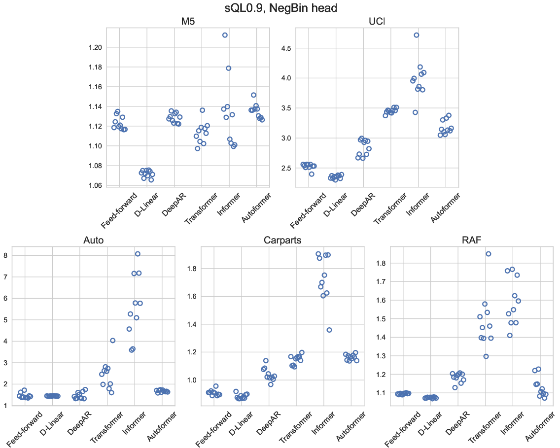
Figure 3: Scaled quantile loss (q=0.9) for global models with negative binomial output, highlighting deep models' instability and inferior accuracy versus simpler alternatives.

Neural Network Architecture Benchmarking

A rigorous ANOVA analysis reveals that D-Linear consistently outperforms both FNNs and DeepAR across most datasets, achieving lower quantile losses, higher stability, and drastically reduced training and inference cost—even as datasets vary in length, intermittency, and volatility:

• FNNs: Consistently underperform relative to D-Linear.
• DeepAR: More competitive, but still less accurate and less efficient than D-Linear.
• D-Linear: Delivers the best overall forecast accuracy, especially for typical quantiles and mean predictions, with minimal run-to-run instability.

This advantage is attributed to the model's moving average (denoising) operation and the reduced risk of overfitting under heavily intermittent conditions.

Distribution Head Evaluation

Tweedie heads excel at predicting extreme quantiles (0.99 and above), as expected given their tail flexibility. However, negative binomial heads remain the most robust choice overall, with neither Tweedie nor HSNB able to provide clear, consistent improvements across all settings. Selection via application-relevant quantile cross-validation is recommended.

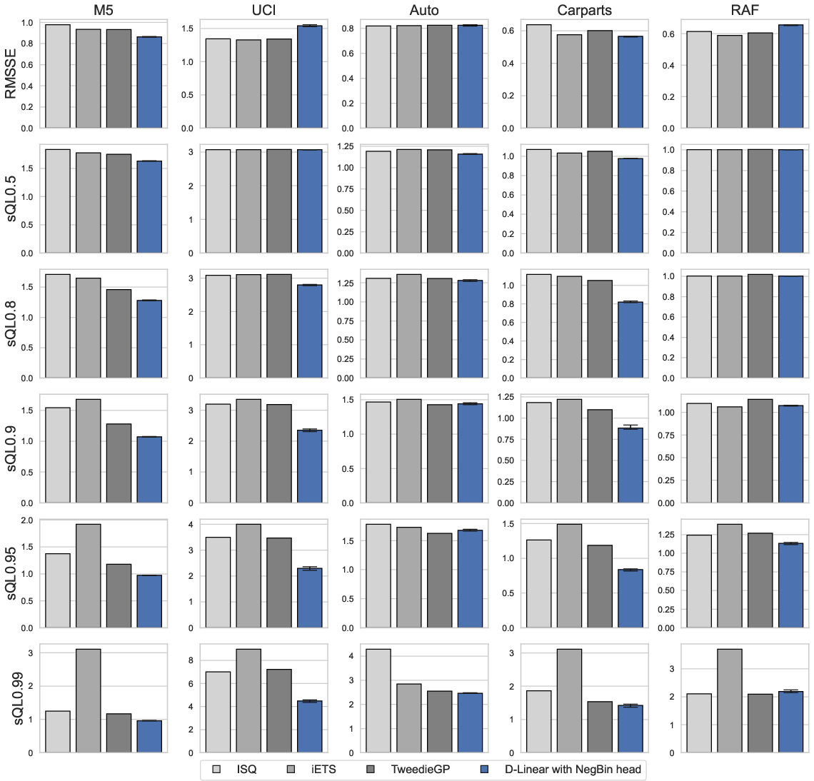
Figure 4: Local model comparison with D-Linear (negative binomial head): D-Linear is superior across most quantile losses, but certain local models match or outperform for highly volatile, very short, or highly sparse series.

Local vs Global Models

Global D-Linear models consistently and significantly outperform local methods (iETS, TweedieGP, ISQ) for the majority of conditional quantiles of interest, particularly as series become longer and less volatile. TweedieGP is a strong local baseline for extreme quantile forecasts and shorter, more volatile series; ISQ remains surprisingly effective in extremely sparse, bursty contexts. However, the D-Linear architecture's speed and accuracy dominate in mainstream settings.

Hyperparameter and Context Sensitivity

D-Linear maintains strong performance even as context window length varies—the model is relatively insensitive as long as context is not excessively short, with negligible benefit to extending context across the entire series.

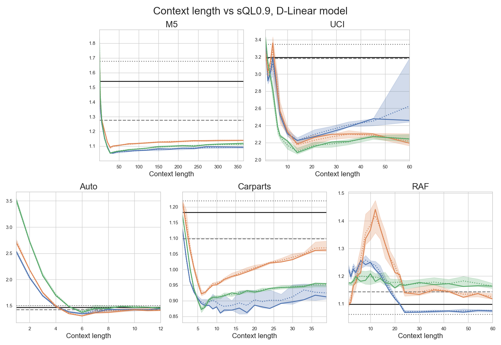
Figure 5: D-Linear performance with varying context length, showing plateaued accuracy after modest context is reached.

Practical and Theoretical Implications

• Global models are not only viable, but superior, for probabilistic intermittent time series forecasting. Their advantage expands as data sets grow and become less volatile or less sparse.
• Deep architectures, notably transformers, add substantial computational burden with little or no accuracy gain for intermittent demand forecasting.
• Model selection for output distribution (forecast head) is nuanced: negative binomial is a robust default; Tweedie is justified for max-quantile optimization or for continuous intermittent targets.
• Shallow, interpretable, and computationally efficient models (e.g., D-Linear) are preferable for practical large-scale applications with hundreds to thousands of intermittent series.
• For datasets or applications exhibiting high volatility, extreme burstiness, short series, or very limited data, simple local approaches remain competitive.

Future Directions

• Explicitly incorporating exogenous variables, hierarchical structure, or leveraging recent advances in parameter-efficient architectures may yield further improvements.
• Extension to real-valued intermittent series (e.g., monetary demand) justifies further study of flexible continuous output heads, such as Tweedie and extensions thereof.
• Further evaluation is warranted for LLM-based sequence models (LLMs applied to time series), which are not included here but represent an emerging and controversial direction.
• Sophisticated hyperparameter optimization or regularization may marginally improve deep model performance but would likely exacerbate their computational and stability issues.

Conclusion

This study establishes that carefully constructed global models—most notably the computationally efficient D-Linear architecture—provide the most reliable and practical probabilistic forecasts for intermittent time series. The findings advocate against the routine use of complex transformer or deep recurrent models in such contexts and recommend negative binomial or Tweedie distribution heads selected by principled cross-validation for application-tailored quantile optimization. These conclusions advocate a paradigm shift in intermittent time series forecasting practice toward scalable, stable, and interpretable global methods.