Grow with the Flow: 4D Reconstruction of Growing Plants with Gaussian Flow Fields
Abstract: Modeling the time-varying 3D appearance of plants during their growth poses unique challenges: unlike many dynamic scenes, plants generate new geometry over time as they expand, branch, and differentiate. Recent motion modeling techniques are ill-suited to this problem setting. For example, deformation fields cannot introduce new geometry, and 4D Gaussian splatting constrains motion to a linear trajectory in space and time and cannot track the same set of Gaussians over time. Here, we introduce a 3D Gaussian flow field representation that models plant growth as a time-varying derivative over Gaussian parameters -- position, scale, orientation, color, and opacity -- enabling nonlinear and continuous-time growth dynamics. To initialize a sufficient set of Gaussian primitives, we reconstruct the mature plant and learn a process of reverse growth, effectively simulating the plant's developmental history in reverse. Our approach achieves superior image quality and geometric accuracy compared to prior methods on multi-view timelapse datasets of plant growth, providing a new approach for appearance modeling of growing 3D structures.

Paper Prompts
Sign up for free to create and run prompts on this paper using GPT-5.
Top Community Prompts
Explain it Like I'm 14
What is this paper about?
This paper is about building a smooth, time-lapse 3D “movie” of a plant as it grows. The authors show a new way to reconstruct how a plant’s shape changes over time from many photos taken around the plant at different moments. Their method, called GrowFlow, focuses on getting the geometry (the actual 3D shape) right as the plant sprouts, expands, and forms new parts.
What questions did the researchers ask?
- How can we make a 3D model that changes over time to show plant growth, not just motion?
- How can we add new plant structures (like new leaves or branches) in a smooth, believable way?
- Can we keep the same 3D parts connected through time so we can track how each part grows?
- Will this approach make better-looking images and more accurate 3D shapes than existing methods?
How did they do it?
Building the plant with 3D “blobs”
Imagine the plant is built from lots of tiny, soft 3D blobs—like fuzzy marbles—each with a position, size, orientation, and color. This idea comes from “3D Gaussian splatting,” a technique that represents scenes using many overlapping, semi-transparent blobs that can be quickly rendered into images from different camera angles.
Modeling growth as a smooth “flow”
Growth isn’t just moving things around; it’s about changing shape over time in a smooth, continuous way. The authors model growth with a “flow field,” which is like a set of instructions telling each blob how to move, rotate, and change size at every moment. Think of it like a gentle, guided breeze that tells each blob how to evolve smoothly over time.
Under the hood, they use something called a neural ODE (ordinary differential equation). You can think of an ODE as a rulebook that says, “Given where a blob is now, here’s how it should change next.” By following these rules step-by-step, you get a continuous animation of the plant’s growth.
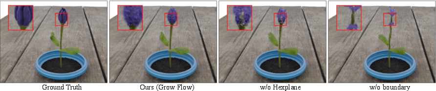
To help the ODE learn smooth changes in space and time, they use a “HexPlane encoder,” which is like a smart, multi-layered 3D+time grid that stores features about the plant’s shape and motion. This makes it easier for the model to produce stable, consistent growth over time.
The clever “reverse-growth” trick
Adding brand-new blobs as the plant grows is hard to optimize (it’s like trying to add LEGO pieces while the model is already moving—it breaks the math). So the authors do something clever: they start from the fully grown plant (the last time point) and learn how it would “shrink” backward in time. In reverse, blobs smoothly get smaller or tuck inside existing parts. Because shrinking is smooth and differentiable, the model can learn it well. Then, when you play the learned process forward, you get realistic, continuous growth.
In simple terms: they learn how to rewind growth, then press play to get the forward growth.
Training in steps to keep things stable
Training a model to handle the entire time-lapse at once can get messy. So they:
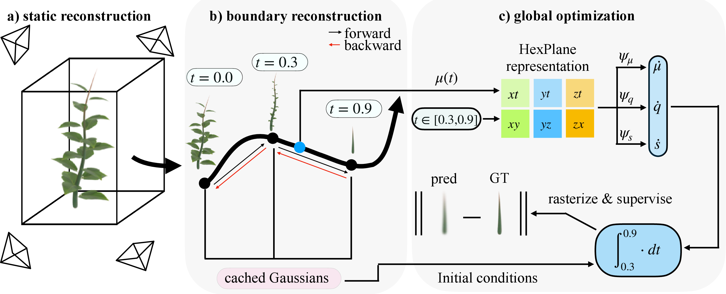
- First, reconstruct the final, fully grown plant as a static 3D blob model.
- Then, step backward one time point at a time, caching (saving) the state at each step—this “boundary reconstruction” keeps the math stable and avoids errors piling up.
- Finally, they do a global pass where they randomly pick time steps and make sure the forward growth matches the real images.
Datasets and tests
They tested on:
- Synthetic (computer-made) plant scenes in Blender, with many views and time steps, so they could measure accuracy precisely.
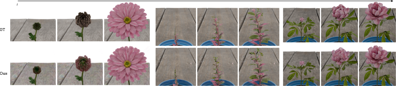
- Real plants (a blooming flower and a corn plant) captured with a camera on a rotating platform, taking photos from all around at many moments.
They compared GrowFlow against several leading methods that model dynamic 3D scenes.
What did they find and why it matters?
Here are the main results:
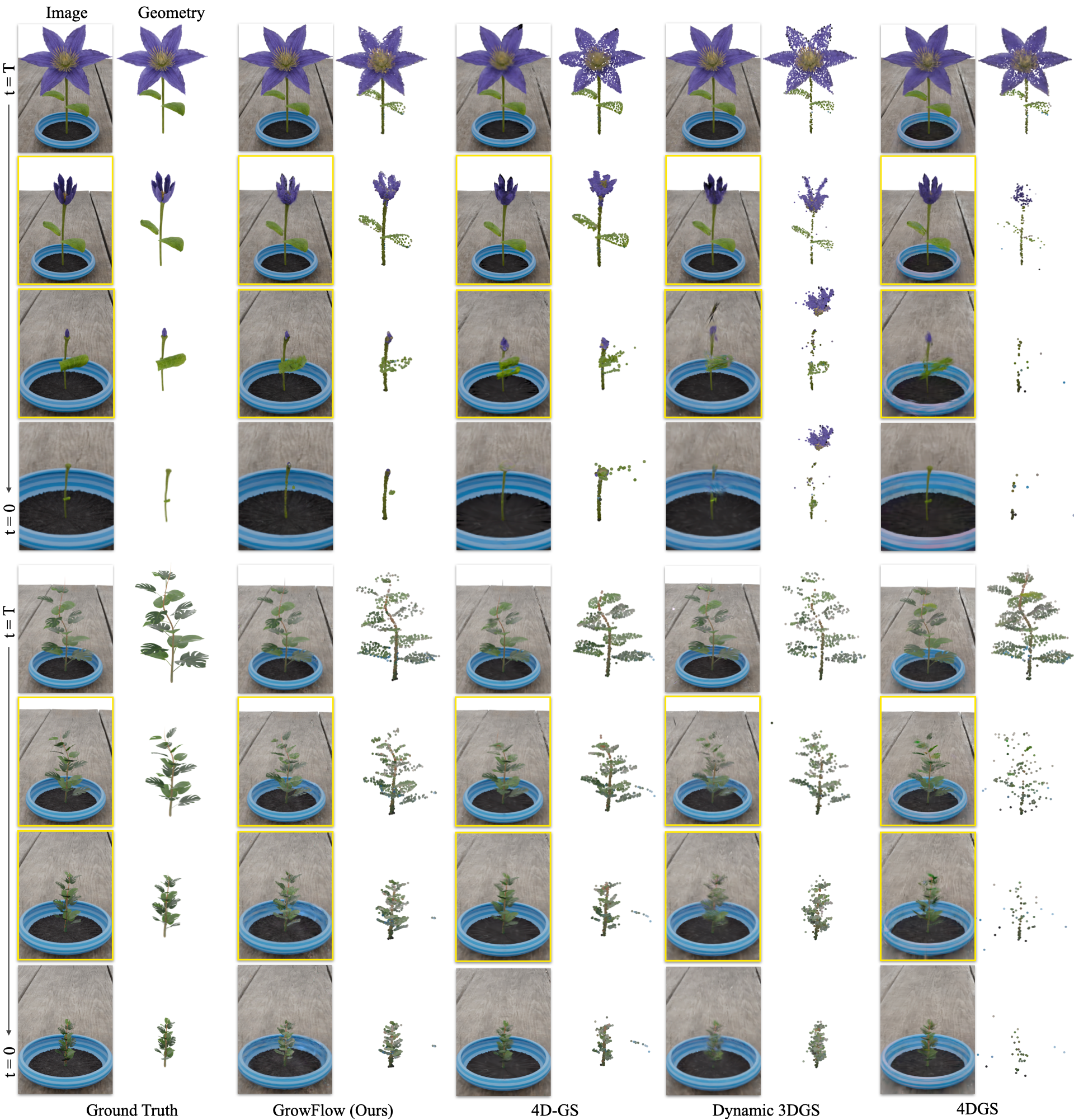
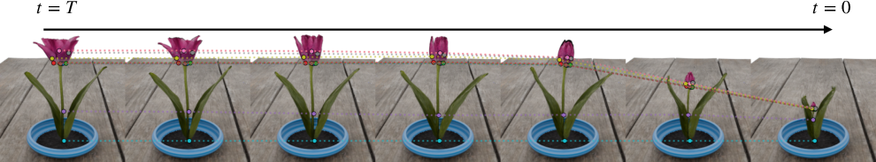
- GrowFlow produced sharper, more accurate 3D shapes of plants as they grew. The blobs stayed attached to the plant’s surface instead of drifting off or wobbling in space.
- It made better-looking images from new viewpoints and at new times (not just the frames it trained on). This is important because real growth is continuous, and the model needs to fill in the gaps between captured moments.
- On synthetic data, GrowFlow clearly beat other methods in both image quality (metrics like PSNR, SSIM, LPIPS) and 3D shape accuracy (measured by Chamfer Distance, which checks how close the reconstructed shape is to the true shape).
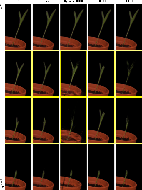
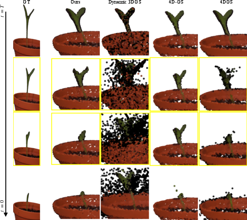
- On real data, GrowFlow stayed stable during “in-between” times where other methods often failed (plants looked like they were growing and shrinking oddly).
This matters because tracking how each part of a plant grows over time is crucial for plant science and agriculture. GrowFlow keeps consistent 3D parts across time, so you can follow a leaf or stem through different stages without losing track.
Why is this important? Future impact
GrowFlow can help:
- Plant phenotyping: Scientists can measure growth patterns more precisely, seeing how leaves and stems expand over time.
- Agriculture: Farmers and researchers can analyze how plants respond to environments (light, water, nutrients) by studying growth in 3D.
- Education and visualization: It creates clear, smooth 3D time-lapses that show plant development in an intuitive way.
Looking ahead, the authors note that they focused on “monotonic” growth—plants only add structure and don’t lose parts. Real plants can also wilt, shed leaves, or get pruned. In the future, the approach could be extended to handle decay or disappearing structures. The same idea could also be applied to other growing things, like crystals forming, embryos developing, or even geological features changing over time.
In short: GrowFlow gives us a reliable, smooth way to watch and measure 3D growth, frame by frame, helping both science and practical applications.
Knowledge Gaps
Knowledge gaps, limitations, and open questions
Below is a single, consolidated list of the key unresolved issues, uncertainties, and missing explorations identified in the paper. Each item is stated concretely to guide future research.
- Monotonic growth assumption: the method cannot handle non-additive dynamics such as senescence, pruning, decay, or transient structures. Develop models that support birth and death processes, reversible growth, and shrinking beyond occlusion.
- Fixed appearance over time: color and opacity are held constant, limiting applicability under changing illumination, pigmentation, translucency, or material properties. Extend to time-varying appearance (opacity, BRDF, SH coefficients) and lighting.
- Dependence on a complete, fully-grown final state: reverse-growth presumes all future geometry exists at . Investigate differentiable, optimizable mechanisms for Gaussian birth/splitting during forward growth when final-state coverage is incomplete or occluded.
- No explicit topology operations: Gaussians neither split nor merge; branching and organogenesis are represented only via motion and scaling. Design differentiable split/merge operations to capture topological changes explicitly.
- Lack of biological/physical priors: growth is learned purely from photometric supervision. Integrate priors (e.g., monotonic volume/area constraints, internode elongation, curvature/strain limits, phyllotaxis rules) and evaluate their impact on plausibility.
- Monotonicity not enforced or measured: although desired, the model does not impose or quantify non-decreasing visible volume forward in time. Define differentiable monotonicity losses and temporal-coherence metrics, and validate them.
- Rotation integration details: quaternion dynamics can drift off the unit sphere or exhibit numerical instability. Analyze and compare stable rotation parameterizations (e.g., exponential map, axis–angle, Lie-group integration) and renormalization strategies.
- ODE solver choices and stability: adjoint method and tolerances are fixed without sensitivity analysis. Systematically study solver types (e.g., RK variants, adaptive methods), tolerances, step sizes, and their trade-offs in accuracy, stability, and runtime.
- Boundary reconstruction reliance: piecewise integration and cached states stabilize training but may introduce subtle discontinuities or bias. Quantify continuity across boundaries and propose regularizers or curriculum strategies that mitigate boundary artifacts.
- Final-timestep degradation: the last frame was excluded from evaluation due to poor quality, indicating end-condition issues. Diagnose causes (overfitting, solver error, cache mismatch) and develop boundary-aware losses or schedule to preserve extreme timesteps.
- Geometry evaluation limited to synthetic data: Chamfer Distance relies on ground-truth meshes, unavailable for captured scenes. Develop real-scene geometry metrics (e.g., multi-view stereo, calibrated fiducials, depth sensors) to validate geometric accuracy.
- Robustness to pose/calibration noise: performance under camera pose errors, intrinsics drift, or turntable misalignment is not assessed. Add joint pose refinement and conduct sensitivity analyses to typical capture imperfections.
- In-the-wild generalization: experiments use controlled turntable setups with static backgrounds. Test on handheld, outdoor, or greenhouse data with dynamic backgrounds, wind-driven motion, occlusions, and diurnal lighting changes.
- Occlusion reasoning: no explicit visibility modeling prevents Gaussians from being “pushed behind” backgrounds during reverse shrinkage. Incorporate differentiable visibility/occlusion losses and background segmentation to prevent non-physical displacements.
- Forecasting beyond observed times: interpolation is demonstrated, but extrapolation (predicting future growth or reconstructing earlier unobserved stages) is not evaluated. Assess forecasting capabilities and uncertainty quantification.
- Dataset scale and diversity: only seven synthetic and two captured scenes with limited morphologies, durations, and complexities. Curate a larger, diverse benchmark (species, growth forms, branching complexity, temporal spans) and report statistical significance.
- Computational efficiency and scalability: training/inference runtimes, memory footprint, and scaling with number of Gaussians, views, and timesteps are not reported. Profile and optimize the pipeline; explore sparse solvers and batched integration.
- Encoder design space: HexPlane outperforms a single MLP in ablation, but other encoders (TriPlanes, K-Planes, multi-resolution hash grids, hybrid implicit–explicit fields) are unexplored. Compare capacity, speed, and stability across encoders.
- Hyperparameter sensitivity: resolutions, number of levels, ODE step sizes, losses, and cache schedules lack sensitivity analysis. Provide guidelines or auto-tuning strategies to improve reproducibility and robustness.
- Material and translucency changes: leaves often thicken, become waxy, or change translucency during growth. Extend the model to time-varying opacity and scattering properties to capture these physical changes.
- Collision and self-intersection: no constraints prevent Gaussians from interpenetrating or producing non-physical overlaps. Add geometric regularizers (self-penetration penalties, collision avoidance) and evaluate their effect.
- Baseline comparison fairness: Dynamic 3DGS interpolation via polynomial fitting may disadvantage the baseline relative to methods natively supporting continuous time. Reassess baselines using their recommended procedures or retraining regimes for temporal interpolation.
- Multi-subject scenes: interactions among multiple plants (competition, occlusion, entanglement) are not addressed. Extend to multi-object growth with shared or interacting flow fields.
- Partial visibility and occluded early structures: early timesteps may include organs later abscised or hidden at , violating reverse-growth assumptions. Investigate bidirectional training (forward and backward flows), partial birth models, or hybrid densification.
- Downstream phenotyping: growth trajectories are not linked to biological measurements (e.g., leaf area index, growth rate maps, internode lengths). Demonstrate integration with quantitative phenotyping tasks and validate against manual annotations.
Practical Applications
Immediate Applications
Below is a set of concrete, deployable use cases that leverage the paper’s findings and method (GrowFlow: 3D Gaussian flow fields with neural ODEs) under the assumptions of multi-view, time-lapse capture with relatively fixed lighting and predominately monotonic plant growth.
- High-throughput 4D plant phenotyping in controlled environments
- Sector: Agriculture, Academia
- Application: Extract temporally coherent traits (leaf emergence timing, branching angles, curvature, growth rate, surface area/volume expansion) from multi-view time-lapse sequences in greenhouses/growth chambers.
- Tools/Workflows: Raspberry Pi + motorized turntable capture rig; gsplat-compatible reconstruction + trait-extraction scripts; HexPlane-ODE training pipeline; visualization dashboards for time-series morphology.
- Assumptions/Dependencies: Reliable multi-view pose calibration; stable, fixed lighting; monotonic growth (no senescence/pruning); sufficient GPU resources; consistent imaging protocol.
- Continuous geometric tracking for morphogenesis research
- Sector: Academia (plant biology, biomechanics)
- Application: Establish dense, temporally coherent 3D correspondences of leaves/stems to study development; quantify local growth vectors; validate or calibrate morphogenesis/biomechanical models.
- Tools/Workflows: GrowFlow reconstruction + per-primitive tracking; export to mesh/point correspondences; integration with analysis notebooks (e.g., Python, MATLAB).
- Assumptions/Dependencies: Controlled imaging; constant color/opacity; ODE solver tolerances tuned for stability.
- Digital content creation and visualization of real plant growth
- Sector: Media/VFX, Education
- Application: Produce photorealistic, temporally coherent growth animations from real plants or synthetic scenes; interactive teaching modules for botany courses.
- Tools/Workflows: Blender/Unreal plugins wrapping GrowFlow; pipeline to render 6-DoF time-lapse sequences; web-based viewers.
- Assumptions/Dependencies: Multi-view timelapse data or artist scenes; GPU rendering; basic 3DGS expertise.
- Horticultural robotics motion planning around delicate structures
- Sector: Robotics, Agriculture
- Application: Use accurate 4D geometry to plan manipulation paths (e.g., tying, staking, micro-pruning) that avoid emerging shoots or buds; schedule actions when geometry is favorable.
- Tools/Workflows: GrowFlow-enabled 4D scene models; robot path planners ingesting dynamic 3D geometry; safety envelopes informed by growth vectors.
- Assumptions/Dependencies: Indoor capture setups; timely reconstruction latency; integration with robot perception stack.
- Nursery quality control and grading
- Sector: Agriculture (nurseries)
- Application: Automate grading via growth trajectory metrics (e.g., uniformity, branching symmetry, target size by time) for early stock selection and quality assurance.
- Tools/Workflows: Batch capture rig; GrowFlow reconstructions feeding QC dashboards; standardized thresholds for pass/fail grading.
- Assumptions/Dependencies: Consistent imaging; controlled environment; agreed-upon trait definitions.
- Maker-grade plant growth kits for hobbyists and educators
- Sector: Daily life, Education
- Application: Affordable DIY kit to capture, reconstruct, and visualize a plant’s 4D growth at home or in classrooms.
- Tools/Workflows: Raspberry Pi + turntable + basic lighting; preconfigured GrowFlow scripts; mobile/web viewer for time-lapse playback and simple metrics.
- Assumptions/Dependencies: Small indoor plants; basic assembly and calibration; limited environmental variability.
- Reproducible phenotyping protocols and benchmark datasets
- Sector: Academia, Policy (standards)
- Application: Use the paper’s synthetic and captured datasets and protocol to standardize multi-view time-lapse phenotyping benchmarks and evaluation metrics (PSNR/SSIM/LPIPS + Chamfer-based geometry).
- Tools/Workflows: Protocol checklists; dataset release; evaluation harness; community challenges.
- Assumptions/Dependencies: Community adoption; shared imaging guidelines; open-source tooling (gsplat, torchdiffeq).
Long-Term Applications
The following applications require further research, scaling, or development (e.g., robust outdoor capture, relaxed assumptions, integration with predictive crop models, real-time pipelines).
- Field-scale 4D crop monitoring with heterogeneous cameras/drones
- Sector: Agriculture, Policy (food security)
- Application: Extend GrowFlow to robustly reconstruct plant growth under variable lighting/weather, occlusions, and sparse/irregular viewpoints; derive trait maps at plot/field scale for yield forecasting and management.
- Tools/Workflows: Multi-agent capture (ground cameras + drones); outdoor-ready photometric normalization; pose/SLAM integration; scalable training/distributed inference.
- Assumptions/Dependencies: Relaxed monotonic growth and fixed-appearance assumptions; advanced radiometric calibration; robust view registration; compute at scale.
- Breeding programs: genotype–phenotype association via 4D traits
- Sector: Agriculture, Academia
- Application: Large-cohort deployment to link genetic variants to fine-grained temporal growth traits; accelerate selection for resilience, yield, and architecture.
- Tools/Workflows: High-throughput imaging pipelines; automated GrowFlow batch processing; statistical genetics modules; data governance/metadata standards.
- Assumptions/Dependencies: Significant infrastructure; standardized trait ontologies; privacy/compliance for data sharing.
- Early stress, nutrient deficiency, and disease anomaly detection
- Sector: Agriculture, Policy (sustainability targets)
- Application: Train models to detect deviations from expected growth trajectories; trigger interventions (irrigation, fertigation, IPM) to reduce inputs and losses.
- Tools/Workflows: Baseline growth priors per cultivar; anomaly scoring on 4D trajectories; decision-support dashboards with alerting.
- Assumptions/Dependencies: Longitudinal baselines; integration with environmental sensors; validated thresholds to minimize false alarms.
- Real-time greenhouse control via closed-loop growth feedback
- Sector: Energy, Agriculture
- Application: Use near-real-time 4D geometry to tune climate setpoints (light, CO₂, temperature) and resource delivery; optimize energy use and growth uniformity.
- Tools/Workflows: Streamed reconstructions; control policies linked to growth metrics; edge inference accelerators.
- Assumptions/Dependencies: Fast capture/reconstruction; robust latency; interoperability with greenhouse control systems.
- Predictive digital twins for scheduling pruning, staking, and harvesting
- Sector: Robotics, Agriculture, Retail Horticulture
- Application: Forecast near-future geometry to plan interventions, reduce damage risk, and optimize labor schedules.
- Tools/Workflows: Forecasting modules built on the learned flow field; task schedulers; human-in-the-loop validation.
- Assumptions/Dependencies: Accurate short-term prediction; modeling of non-monotonic events (senescence, pruning); uncertainty quantification.
- Consumer-grade smartphone capture with monocular or sparse views
- Sector: Daily life, Consumer Software
- Application: Relax multi-view requirements to single or few-view videos using learned priors; democratize 4D plant reconstructions for hobbyists.
- Tools/Workflows: Mobile app; cloud or on-device inference; pose estimation and learned regularizers; lightweight HexPlane alternatives.
- Assumptions/Dependencies: Robustness to limited views and variable lighting; model generalization; efficient mobile inference.
- Regulatory and insurance use: auditable 4D evidence for crop claims
- Sector: Finance, Policy
- Application: Use time-stamped 4D reconstructions to substantiate growth progress, stress events, or losses for insurance and compliance audits.
- Tools/Workflows: Tamper-evident logging; standardized reporting formats; secure data retention policies.
- Assumptions/Dependencies: Accepted standards; legal frameworks; privacy and provenance requirements.
- Integration with biophysical and mechanistic growth models
- Sector: Academia, Agriculture
- Application: Fuse GrowFlow’s empirical geometry with mechanistic models (e.g., L-systems, biomechanics, photosynthesis models) for causally grounded simulations and hypothesis testing.
- Tools/Workflows: Hybrid pipelines combining ODE-based flow with physiological simulators; parameter estimation; sensitivity analyses.
- Assumptions/Dependencies: Model identifiability; accurate environmental covariates; cross-disciplinary tooling.
- Biodiversity and urban greening monitoring (seedlings, saplings)
- Sector: Environmental Policy, Urban Planning
- Application: Track establishment success and growth of urban plantings; evaluate interventions’ impact; guide species selection for resilience.
- Tools/Workflows: Periodic multi-view capture; municipal analytics dashboards; standardized ecological indicators derived from 4D geometry.
- Assumptions/Dependencies: Outdoor robustness; diverse species morphology; scalable city deployments.
- Cross-domain extensions to emerging geometry (beyond plants)
- Sector: Materials (crystal growth), Medicine (embryogenesis), Geoscience
- Application: Adapt the flow-field approach to other systems where geometry emerges over time; unify reconstruction and analysis workflows for dynamic structure formation.
- Tools/Workflows: Domain-specific capture setups (microscopy, medical imaging); tailored appearance/physics priors; validation datasets.
- Assumptions/Dependencies: Appropriate imaging modalities; domain-specific relaxation of fixed appearance and monotonicity assumptions.
Common Assumptions and Dependencies Across Applications
- Monotonic growth assumption: Current method presumes non-decreasing visible volume; extension needed to handle senescence, pruning, decay.
- Fixed appearance: Color/opacity are modeled as time-invariant; outdoor or developmental color changes require model adaptation.
- Capture constraints: Requires multi-view, time-lapse imaging with reliable pose estimation; controlled lighting improves fidelity.
- Compute and expertise: GPU resources, 3DGS/ODE solver know-how (e.g., torchdiffeq, gsplat), and calibration pipelines are necessary.
- Data governance: For scaled deployments (breeding, insurance, policy), standards for metadata, privacy, and reproducibility are critical.
Glossary
- 3D Gaussian Splatting (3DGS): A real-time rendering technique that represents scenes with many anisotropic 3D Gaussian primitives optimized from multi-view images. "Recently, 3D Gaussian Splatting (3DGS)~\cite{kerbl20233d} has emerged as a powerful scene representation technique"
- 4D Gaussian Splatting (4D-GS): A dynamic extension of 3DGS for time-varying scenes, optimizing Gaussian parameters across space-time. "Notably, 4D-GS \cite{wu20244d} completely fails during interpolation where the reconstructed plant wobbles between growing and shrinking"
- 4DGS: Another 4D Gaussian-based dynamic scene representation with temporal masking to handle changing visibility. "For 4DGS, we apply their temporal masking before computing distances."
- Adam optimizer: A stochastic gradient-based optimization algorithm widely used for training neural networks. "For static reconstructions of fully grown plants, we use 3DGS with default training settings and the Adam~\cite{kingma2014adam} optimizer"
- Adjoint method: A technique for efficiently computing gradients through ODE solvers during training of Neural ODEs. "During the boundary reconstruction phase, we optimize each boundary timestep for 300 iterations using the adjoint method~\cite{chen2018neural}"
- Alpha blending: A compositing process that blends primitives along depth using their opacity to produce the final image. "and then alpha-blended in depth order to render the target image."
- Bilinear interpolation: A method to interpolate values on 2D grids (planes), here used across spatial-temporal planes for continuous features. "Features are bilinearly interpolated from the six spatio-temporal planes "
- Boundary reconstruction: A staged training process that reconstructs intermediate time boundaries to stabilize ODE integration. "During the boundary reconstruction phase, we optimize each boundary timestep for 300 iterations"
- Cached boundary states: Stored Gaussian configurations at intermediate timesteps used as initial conditions for subsequent integration. "After each reconstructed timestep, we cache the Gaussians for that timestep and use them as initial conditions to optimize for the next timestep."
- Canonical space: A reference configuration to which deformation fields map to produce per-timestep states. "Contemporary dynamic scene models often rely on deformation fields that map a canonical space to a deformed state at each timestep"
- Chamfer Distance (CD): A symmetric distance metric between two point sets, used here to assess geometric fidelity across time. "We introduce a 3D point-tracking metric based on the Chamfer Distance (CD)."
- Continuous dynamical system: A formulation where scene evolution is governed by smooth time-continuous transformations. "We propose a new perspective: plant growth can be modeled as a continuous dynamical system"
- Deformation fields: Functions that warp a canonical representation into observed states; they preserve topology and cannot add new geometry. "deformation fields preserve topologyâthey can only move existing points in spaceâand therefore cannot directly introduce new geometry."
- Densification: Increasing the number or density of primitives; in 3DGS this is discrete and non-differentiable. "Conversely, densification in 3DGS is a discrete, non-differentiable process"
- Flow field: A vector field over parameters that defines their time-evolving dynamics; here, over Gaussian parameters. "a flow field defined over their parameters"
- Gaussian primitives: The basic scene elements in 3DGS, each with position, scale, orientation, color, and opacity. "using a set of 3D Gaussian primitives"
- HexPlane encoder: A spatio-temporal grid representation that interpolates features across six planes to efficiently encode dynamics. "We model the velocity field using a spatio-temporal HexPlane encoder"
- L1 loss: The mean absolute error metric used for supervising reconstructions alongside SSIM. "optimizing a mixture of L1 and SSIM losses."
- Latent feature: A learned intermediate representation extracted from HexPlane interpolation for decoding velocities. "we extract a latent feature via:"
- Linearized projection model: An approximation used to project 3D Gaussians to views for rasterization. "These Gaussians are projected into a given view using a linearized projection model~\cite{zwicker2001ewa}"
- LPIPS: A learned perceptual image similarity metric for evaluating photometric quality. "PSNR, LPIPS, and SSIM."
- MLP (multi-layer perceptron): A feed-forward neural network used to decode velocities from latent features. "followed by multi-layer perceptron (MLP) decoders"
- Monotonic growth: A constraint that the visible volume should not decrease over time during reconstruction. "while ensuring that the visible volume of the plant is monotonically non-decreasing"
- Neural field: A continuous function (often parameterized by a neural network) mapping coordinates to scene properties; here time-integrated for dynamics. "We then develop a time-integrated neural field"
- Neural ODEs: Neural networks that parameterize the right-hand side of ODEs, enabling learned continuous-time dynamics. "Neural ODEs~\cite{chen2018neural} parametrize the underlying flow field using a neural network and recover the trajectory of the system by integration."
- Novel-view synthesis: Rendering accurate views from unseen camera poses, extended here to novel timesteps. "Our approach retains high-fidelity geometry and achieves state-of-the-art performance in both novel-view and novel-time synthesis."
- Numerical ODE solver: An algorithm to integrate ODEs (e.g., Runge–Kutta), recovering parameter trajectories across time. "which can be solved using standard numerical ODE solvers such as RungeâKutta~\cite{butcher1996history,runge1895,kutta1901}."
- Occlusion: The process by which structures become hidden behind others in the rendered scene. "or by becoming occluded within existing matter."
- Ordinary differential equation (ODE): A mathematical model describing continuous-time rate of change of system states. "In the continuous-time limit, such dynamics can be described by an ordinary differential equation (ODE)."
- Piecewise integration: Integrating ODEs over short segments between cached boundaries to improve stability. "we adopt a piecewise integration strategy"
- Point cloud registration: Aligning 3D point sets across time; prior plant methods used this instead of continuous Gaussian dynamics. "these methods rely on point cloud registration rather than modeling continuous-time dynamics with 3D Gaussians"
- PSNR: Peak Signal-to-Noise Ratio, an image fidelity metric used to evaluate reconstruction quality. "PSNR, LPIPS, and SSIM."
- Quaternion (rotation quaternion): A four-dimensional representation of 3D rotations used to parameterize Gaussian orientation. "rotation quaternion "
- Rasterization: Converting parametric primitives (Gaussians) into pixel values for image supervision. "The predicted Gaussians are then rasterized and supervised"
- Reverse growth: Training by shrinking from the final state backward in time, then reversing the learned flow to obtain forward growth. "we reconstruct the mature plant and learn a process of reverse growth"
- Runge–Kutta: A family of numerical methods for solving ODEs used to integrate Gaussian parameter dynamics. "such as RungeâKutta~\cite{butcher1996history,runge1895,kutta1901}"
- Slerp (spherical linear interpolation): A method to smoothly interpolate rotations on the unit quaternion sphere. "Rotations are interpolated using spherical linear interpolation (slerp)"
- Spherical harmonics: Basis functions on the sphere used to represent view-dependent color coefficients. "represented via rank- spherical harmonics."
- SSIM: Structural Similarity Index, an image quality metric assessing perceived structural fidelity. "optimizing a mixture of L1 and SSIM losses."
- Spatio-temporal Gaussians: Gaussian primitives parameterized across space and time to capture dynamics. "Another line of work optimizes 4D spatio-temporal Gaussians to represent the sceneâs evolution~\cite{yang20244d, duan20244d, li2024spacetime}."
- Temporal masking: A mechanism that activates/deactivates Gaussians over time to handle changing visibility. "using 4D Gaussians combined with temporal masking mechanisms~\cite{li2024spacetime, duan20244d, yang20244d}"
- Time-lapse imagery: Sequences of images captured over time to observe gradual changes like plant growth. "Given multi-view timelapse images of a plant"
- Topology: The connectivity and arrangement of geometric elements; preserved by deformations but not changed to add new parts. "deformation fields preserve topologyâthey can only move existing points in spaceâand therefore cannot directly introduce new geometry."
- Velocity field: A function giving instantaneous rates of change (translation, rotation, scale) of Gaussian parameters over time. "We define a time-dependent velocity field governing the dynamics of each Gaussian"
- Vector field: A field assigning a vector (direction and magnitude) to each point; here, governing growth dynamics in parameter space. "This formulation captures the underlying growth vector field"
Collections
Sign up for free to add this paper to one or more collections.