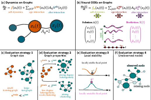
When do neural ordinary differential equations generalize on complex networks?
Abstract: Neural ordinary differential equations (neural ODEs) can effectively learn dynamical systems from time series data, but their behavior on graph-structured data remains poorly understood, especially when applied to graphs with different size or structure than encountered during training. We study neural ODEs ($\mathtt{nODE}$s) with vector fields following the Barabási-Barzel form, trained on synthetic data from five common dynamical systems on graphs. Using the $\mathbb{S}1$-model to generate graphs with realistic and tunable structure, we find that degree heterogeneity and the type of dynamical system are the primary factors in determining $\mathtt{nODE}$s' ability to generalize across graph sizes and properties. This extends to $\mathtt{nODE}$s' ability to capture fixed points and maintain performance amid missing data. Average clustering plays a secondary role in determining $\mathtt{nODE}$ performance. Our findings highlight $\mathtt{nODE}$s as a powerful approach to understanding complex systems but underscore challenges emerging from degree heterogeneity and clustering in realistic graphs.
Paper Prompts
Sign up for free to create and run prompts on this paper using GPT-5.
Top Community Prompts
Explain it Like I'm 14
What is this paper about?
This paper studies a kind of AI model called a “neural ordinary differential equation” (neural ODE) and asks: when can it accurately learn and predict how things change over time on complex networks? Think of a network as a big web of connected points (like people in a social network or computers on the internet), and a dynamical system as rules that describe how each point’s state changes over time because of itself and its neighbors.
What questions did the researchers ask?
The authors explored four simple but important questions about how well neural ODEs work on networks:
- Can a model trained on a small network make good predictions on a much bigger network?
- Can a model trained on networks with certain properties (like how many “hub” nodes there are or how clustered the network is) still work on networks with different properties?
- Does the model correctly learn the system’s steady states (called fixed points) and whether those states are stable?
- How well does the model cope if some parts of the network are hidden or missing at test time?
How did they do it?
The researchers built and tested their models in a carefully controlled, “best case” setup so they could clearly see what helps or hurts performance.
- The model: They used neural ODEs designed to match a simple, common recipe for networked dynamics (called the Barabási–Barzel form). In plain terms, each node’s change over time is split into:
- a self-effect (how it changes on its own), and
- neighbor effects (how connected neighbors push or pull it).
- The model learns these two parts with neural networks.
- The networks: They generated many synthetic (fake but realistic) networks where they could control:
- degree heterogeneity: whether a few nodes are “hubs” with lots of links (more heterogeneity) or most nodes have similar numbers of links (less heterogeneity),
- clustering: how often a node’s friends are also friends with each other (lots of triangles).
- This let them dial in networks that look more or less like real-world systems.
- The systems they modeled: They created training data from five common kinds of dynamics on networks:
- SIS (disease spread),
- MAK (chemical reactions),
- MM (gene regulation),
- BD (birth–death in populations),
- ND (activity in brain regions).
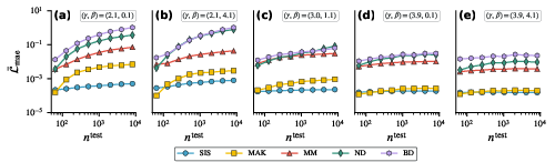
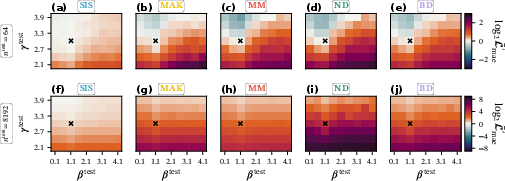
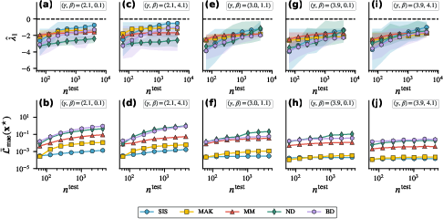
- The tests: They trained on small networks (64 nodes) and then checked: 1) size generalization (up to 8,192 nodes), 2) property generalization (different amounts of hubs and clustering), 3) fixed-point accuracy and stability, 4) robustness when some nodes are unobserved (missing).
They scored predictions using simple error measures (how far off the model’s predictions were from the true values over time).
What did they find, and why is it important?
Here are the main takeaways:
- Degree heterogeneity (hubs) is the biggest challenge for generalization.
- When networks have many hubs, models trained on small graphs struggle on much larger graphs for several of the dynamics (especially MM, ND, and BD). The exception is SIS (and often MAK), which handled scaling better.
- Why? In some systems, the state of high-degree nodes (hubs) gets much larger than what the model saw during training. That forces the model to guess in unfamiliar territory, which hurts accuracy.
- Clustering matters, but less than degree heterogeneity.
- Higher clustering can make things harder, but its effect was usually smaller than the effect of hubs.
- Generalizing to different network properties works best when the new network is simpler than the training one.
- Models trained on networks with moderate properties did fine on networks with fewer hubs and less clustering.
- But accuracy often dropped when moving to more hub-heavy or more clustered networks—especially on large graphs.
- Fixed points: models found stable steady states, but sometimes the wrong ones on hub-heavy networks.
- The models tended to settle into stable behavior (good sign), but in very heterogeneous networks the steady state could differ from the true system’s steady state.
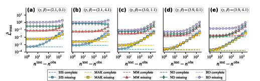
- Missing data makes predictions worse—and how quickly that happens depends on the network and system.
- Even hiding a small number of nodes can increase errors, especially on some dynamics.
- Interestingly, very hub-heavy networks sometimes tolerated more missing nodes because the most important hubs were less likely to be hidden by random removal. But overall, these same hub-heavy networks were already harder to predict well in the first place.
Why this matters: Many real networks (like social, biological, or technological systems) have hubs and clustering. These findings show exactly where neural ODEs shine and where they can fail, helping researchers use them more safely and effectively.
What’s the bigger picture?
- For practice: If you train on small networks and deploy on larger ones, check how “hubby” your networks are. If there are many hubs, collect more diverse training data or design models that can handle extreme node values.
- For evaluation: Don’t only measure short-term prediction error. Also test whether the model learns correct steady states and how robust it is to missing data.
- For future research: Improve model designs to better handle hubs and clustering, and build training strategies that expose models to a wider range of node states. Test on networks with realistic structures (and use network generators that let you tune these structures on purpose).
In short, neural ODEs can be powerful tools for understanding how things change on networks, but their reliability depends on the network’s structure and the type of dynamics. Knowing when and why they generalize—or fail—helps scientists trust and improve these models for real-world problems.
Knowledge Gaps
Unresolved gaps, limitations, and open questions
Below is a concise list of concrete knowledge gaps and limitations identified in the paper that future work could address:
- Generality beyond BB form: The study is restricted to Barabási–Barzel (BB) dynamics with separable interactions; it remains unknown how nODEs perform on non-separable interaction models (e.g., Kuramoto, Laplacian diffusion, SIS with pairwise state differences) and whether architectures with non-factorized interaction parameterizations improve generalization.
- Dynamics parameter generalization: All dynamical system parameters () are fixed during training and testing; how performance and stability change when these parameters vary (including out-of-training-range) is not tested.
- Initial-condition distribution shift: The training initial conditions come from fixed uniform ranges; the ability to generalize to out-of-distribution initial states (beyond the cited prior result) is not systematically assessed for the current architecture and evaluation settings.
- Average degree/sparsity effects: The impact of the average degree (and thus sparsity/density) on generalization, fixed-point fidelity, and robustness is not explored, even though is a core S1-model parameter.
- Real-world networks and mesoscopic structure: Results are derived on S1-model graphs; effects of communities, degree correlations (assortativity), core–periphery, motifs, and other mesoscopic structures commonly found in empirical networks remain untested.
- Directed and weighted graphs: The analysis is limited to simple undirected, unweighted graphs; how directionality and edge weights (including signed weights) affect learning and generalization is unknown.
- Multi-dimensional node states: Only scalar node states are considered; many real systems have vector-valued states (e.g., multi-species, multi-compartment neuronal models). The scalability and accuracy of nODEs with higher-dimensional node states is unassessed.
- Time-varying graphs and non-autonomous dynamics: The setting assumes static graphs and autonomous ODEs; performance under time-varying topologies, exogenous inputs, or explicitly time-dependent vector fields remains unexplored.
- Stochastic dynamics: All systems are modeled deterministically (ODEs); extensions to stochastic dynamics (SDEs or continuous-time Markov processes) and the implications for training, uncertainty, and generalization are not considered.
- Training on a single graph vs. multiple graphs: Models are trained on one graph per regime; whether training on multiple graph realizations (or a curriculum over sizes/properties) improves size and property generalization is not evaluated.
- Sensitivity to training graph size: The study trains on graphs with ; how increasing changes generalization to very large graphs and whether there is a sample/size threshold for reliable hub behavior remains open.
- Solver and stiffness considerations: A single adaptive solver/tolerance is used; sensitivity of training and inference to solver choices, tolerances, and potential stiffness in certain regimes is not quantified.
- Long-horizon prediction: Time windows are fixed (e.g., ); whether errors accumulate over longer horizons and how stable integration is over longer times is not analyzed.
- Constraint adherence and invariants: The architecture does not explicitly enforce physical/biological constraints (e.g., positivity, boundedness for SIS), conservation laws, or monotonicities; whether adding such constraints improves fixed-point accuracy and generalization is untested.
- Interpretability and identifiability: While f, hego, and halt are learned, the paper does not evaluate whether they recover interpretable or unique functions, nor assess identifiability under the factorized parameterization.
- Theoretical understanding: The explanation for size-generalization failures on degree-heterogeneous graphs is heuristic (state magnitude vs. degree); formal bounds linking degree distributions, state ranges, Lipschitz properties, and generalization error are lacking.
- Degree normalization and architectural variants: The architecture sums neighbor contributions without degree normalization; whether degree-normalized interactions, attention mechanisms, or other aggregators mitigate hub-induced OOD issues is not investigated.
- Ablations and capacity controls: The influence of network width/depth, regularization (e.g., weight decay, spectral norm, monotonicity constraints), and activation choices on robustness and generalization is not ablated.
- Baselines and comparative evaluation: No comparisons are provided against alternative graph dynamical models (e.g., discrete-time GNNs, graph neural operators, physics-informed baselines, mechanistic models), leaving relative strengths/weaknesses unclear.
- Uncertainty quantification: The approach is deterministic without uncertainty estimates; calibration, confidence intervals, and predictive uncertainty (especially at hubs or OOD graphs) are not studied.
- Fixed-point landscape: Only the largest Jacobian eigenvalue is examined around a single fixed point; multiple equilibria, basin sizes, global vs. local stability, and bifurcations as graph/dynamics parameters vary are not analyzed.
- Property disentanglement: Clustering is reported to play a “secondary role,” but causal disentanglement between clustering, path length, and motif structure is not provided; mechanisms by which clustering affects performance remain unclear.
- Missingness patterns and edge uncertainty: Missing nodes are sampled uniformly; the impact of structured missingness (degree-, community-, or geography-biased), missing edges, uncertain edges/weights, or partial temporal observations is not explored.
- Training with partial observations: Robustness to missing data is tested only at inference; whether training with masked nodes/edges (or latent-variable models) improves robustness is untested.
- State imputation for unobserved nodes: The study evaluates prediction at observed nodes only; methods and performance for inferring trajectories of unobserved nodes are not examined.
- Transfer to empirical data: The framework is validated on synthetic data; applicability to real datasets (e.g., epidemics on contact networks, gene-regulatory networks, brain connectomes) and the alignment between S1-based insights and empirical behavior remain open.
- Computational scalability: Although inference on large graphs is tested, training-time and memory scaling, solver-step counts, and wall-clock costs across graph sizes/properties are not reported, limiting practical deployment guidance.
- Hyperparameter robustness: Sensitivity to hyperparameters (learning rates, batch sizes, solver tolerances, training noise, number of trajectories) is not systematically assessed.
- Time discretization and sampling frequency: The effect of observation cadence (number and spacing of time points) on identifiability, training stability, and prediction accuracy is not evaluated.
- Edge cases at extreme heterogeneity: In very heavy-tailed degree regimes, the model encounters extreme states at hubs; strategies to avoid extrapolation (e.g., degree-dependent rescaling, clipping, curriculum over degree) are not investigated.
- Generalization diagnostics: There is no explicit OOD detector or degree-aware calibration to flag unreliable predictions on hubs or unseen graph regimes.
- Interaction between clustering and degree heterogeneity: The interplay is summarized empirically; a mechanistic or theoretical explanation for when clustering amplifies or mitigates hub-driven errors is missing.
- Data efficiency: The number of trajectories/time series used for training and how performance scales with training data volume are not analyzed, leaving sample-efficiency questions unresolved.
Practical Applications
Immediate Applications
The paper’s results support several deployable practices, tools, and use cases, especially when network degree heterogeneity is modest and the target dynamics resemble the BB (Barabási–Barzel) form.
- Pre-deployment stress testing for graph-dynamics models
- What to do: Adopt the paper’s four-part evaluation protocol (size generalization, property generalization, fixed-point/stability, missingness robustness) as a standard pre-deployment checklist for any neural ODE (or comparable ML) used on networked systems.
- Sectors: Software/ML Ops, healthcare, energy, telecom, robotics.
- Tools/products/workflows: “nODE Stress-Test Harness” that (i) computes degree heterogeneity (γ) and clustering (β); (ii) generates S1-model graphs to bracket deployment scenarios; (iii) quantifies size-generalization and robustness metrics; (iv) computes Jacobian eigenvalues to check stability.
- Assumptions/dependencies: Access to representative training data; ability to estimate target network’s γ and average clustering; BB-form dynamics or close approximations; static graph during prediction horizon.
- Safe deployment guidelines on moderate-heterogeneity networks
- What to do: Prefer deployments on networks with higher γ (i.e., less degree heterogeneity) and similar clustering to training graphs; prioritize SIS-/MAK-like dynamics where size generalization is empirically strongest.
- Sectors: Building HVAC and microgrid control (energy), service-dependency prediction (software), hospital-ward outbreak modeling (healthcare).
- Tools/products/workflows: Degree- and clustering-aware “model selection” rules-of-thumb in ML pipelines; automated alerts if target γ or β exceeds trained ranges; fallback to simpler models if thresholds are exceeded.
- Assumptions/dependencies: Accurate measurement (or robust estimation) of γ and β for the target graph; dynamics captured reasonably by separable interaction terms.
- Data collection and sensor placement that prioritizes hubs (when feasible)
- What to do: In highly heterogeneous networks (low γ), prioritize observation/sensing of high-degree nodes to mitigate error growth from partial observability; adjust sampling budgets accordingly.
- Sectors: Telecom (network operations), cybersecurity (attack propagation), epidemiology (contact tracing in subpopulations), supply chain monitoring.
- Tools/products/workflows: “Hub-first sensing” policy; active sampling schedules keyed to degree ranks; observability dashboards quantifying predicted error vs. fraction of observed hubs.
- Assumptions/dependencies: Ability to identify (even approximately) high-degree nodes; partial observability is a key constraint; missingness is not strongly adversarial/structured against hubs.
- Fixed-point and stability checks to validate control strategies
- What to do: Use the learned nODE to identify fixed points and check local stability (largest Jacobian eigenvalue < 0), especially on less heterogeneous networks where fixed points are well aligned with ground truth.
- Sectors: Energy (operating point analysis in distribution networks), neuroscience (coarse-grained brain region dynamics), chemical/bioprocess control.
- Tools/products/workflows: “Equilibria Checker” that runs stable fixed-point detection and Jacobian analysis on learned models; tie to control setpoint validation.
- Assumptions/dependencies: Dynamics approximated by BB-form; smaller or less heterogeneous graphs; static graph; sufficient data to fit nODE locally around operational regimes.
- Risk scoring and deployment guardrails for OOD network regimes
- What to do: Compute a “Graph Dynamics Readiness Score” combining (i) mismatch in γ, β vs. training; (ii) expected size jump; (iii) expected missingness; (iv) dynamics class; gate deployments when score exceeds policy thresholds.
- Sectors: Critical infrastructure, finance (systemic risk propagation), public health analytics, IT Ops.
- Tools/products/workflows: Policy-based deployment guardrails integrated in MLOps; dashboards showing expected degradation under size scaling and property shifts.
- Assumptions/dependencies: Reliable estimates of graph properties; enforcement culture for model risk management.
- Synthetic augmentation for robustness within BB-form
- What to do: Augment training with S1-generated graphs spanning a range of γ, β around expected deployment conditions; oversample trajectories involving high-degree nodes to reduce state-space extrapolation.
- Sectors: General ML for networked systems, especially where small training graphs are unavoidable.
- Tools/products/workflows: Curriculum training from smaller to larger S1 graphs; hub-focused data augmentation; weighted loss for high-degree node trajectories.
- Assumptions/dependencies: Simulator access or historical data to seed augmentation; BB-form fidelity; compute budget for augmentation.
- Academic benchmarking and reproducible evaluation
- What to do: Use the provided code and S1-model protocol to benchmark graph-dynamics learners across size/property generalization, stability, and missingness.
- Sectors: Academia and R&D; open-source ML.
- Tools/products/workflows: Standardized benchmark suites; leaderboards that report not only predictive error but also stability and robustness metrics.
- Assumptions/dependencies: Community buy-in; agreement on parameter sweeps and metrics.
Long-Term Applications
Advances here require further research, scaling, or architectural development but can significantly broaden the impact of neural ODEs on complex networks.
- Degree-aware and non-separable interaction architectures
- What to build: nODE variants that (i) explicitly normalize by degree or neighborhood statistics to curb state growth at hubs; (ii) learn non-separable interactions (e.g., Laplacian, Kuramoto-like terms) when BB-form is insufficient.
- Sectors: Power systems (grid stability), brain dynamics, materials/chemical reactors, social contagion with threshold effects.
- Tools/products/workflows: New layers/regularizers that enforce boundedness/monotonicity; contrastive objectives to match fixed points with known physics; architecture search with degree-normalized operators.
- Assumptions/dependencies: Access to physics priors; scalable differentiable solvers; careful numerical stability handling.
- Active sensing and optimal observation for partial graphs
- What to build: Algorithms that decide which nodes to observe to keep prediction error below a target; combine hub prioritization with uncertainty estimates and structural priors.
- Sectors: Telecom monitoring, smart grids, transportation, epidemiological surveillance.
- Tools/products/workflows: “Observer design” modules that integrate with sensor placement; online policies that adapt to graph changes; uncertainty-aware nODEs.
- Assumptions/dependencies: Budgeted sensing; dynamic graphs; integration with field constraints and privacy.
- Foundation models for graph dynamics
- What to build: Pretrained operators on large corpora of simulated S1 graphs and diverse dynamics, enabling zero-/few-shot adaptation to new networks and processes.
- Sectors: Cross-domain scientific ML, digital twins for cities/industry, climate-impact networks.
- Tools/products/workflows: Multi-dynamics pretraining; property-conditioned decoders (conditioning on γ, β, size); adapters for domain-specific constraints.
- Assumptions/dependencies: Large-scale compute and datasets; standardized graph/dynamics metadata; robust OOD detection.
- Robustness certification and regulatory standards
- What to build: Certification protocols for ML-driven simulators of networked systems that mandate tests analogous to the paper’s four strategies; policy frameworks defining acceptable risk bands for deployment.
- Sectors: Critical infrastructure, healthcare, finance, public policy.
- Tools/products/workflows: Compliance toolkits that auto-generate reports on size/property generalization, stability, and missingness; regulator-approved benchmarks.
- Assumptions/dependencies: Interdisciplinary consensus on metrics; regulatory adoption; interpretable reporting.
- Digital twin platforms with property-aware model selection
- What to build: Digital twins that continuously estimate network properties (γ, β) and trigger model retraining or switching when drift is detected; integrate fixed-point alignment checks into control loops.
- Sectors: Smart buildings/campuses, manufacturing lines, power distribution, water networks.
- Tools/products/workflows: “Graph property monitors” in production; automated retraining pipelines; guardrail controllers that leverage stability diagnostics.
- Assumptions/dependencies: Reliable online estimation of graph properties; data versioning; safe-switching strategies.
- Methods to align learned and physical equilibria
- What to build: Training objectives or constraints that force the learned model’s fixed points and their stability to match known equilibria (from domain theory or steady-state measurements).
- Sectors: Chemical and bioprocess engineering, systems biology, power systems.
- Tools/products/workflows: Physics-informed loss terms; equilibrium datasets; post-training equilibrium calibration routines.
- Assumptions/dependencies: Availability of equilibrium annotations; differentiable solvers; identifiability under noise.
- Application to highly heterogeneous real-world networks at scale
- What to build: End-to-end solutions for city-scale epidemiology, systemic risk in finance, Internet traffic dynamics—where degree heterogeneity and clustering are high.
- Sectors: Public health, finance, Internet infrastructure.
- Tools/products/workflows: Heterogeneity-robust architectures; uncertainty quantification; hybrid ML–mechanistic models; scenario stress testing over S1-like envelopes of network properties.
- Assumptions/dependencies: High-fidelity network data; privacy-preserving computation; cross-agency data sharing.
Cross-cutting assumptions and dependencies (impacting feasibility)
- The BB-form (separable interactions, homogeneous node dynamics, static graph) must be a reasonable approximation; otherwise, non-separable or time-varying architectures are needed.
- Node states are scalar in the study; vector-valued states may require richer parameterizations.
- Real networks often have communities, degree correlations, and temporal evolution not captured by the S1 model; evaluations should include domain-specific null models or real networks where possible.
- Training on small graphs transfers best when deployment networks have similar γ, β and dynamics; otherwise, augment or retrain.
- Missingness in practice may be structured (non-random); robustness must be re-evaluated under domain-relevant missingness patterns.
Glossary
- Adjacency matrix: A matrix representing which pairs of nodes in a graph are connected by an edge. "interactions take place along the edges of a graph, encoded in its adjacency matrix A"
- Autonomous system: A system of differential equations without explicit time dependence in its dynamics. "the system of differential equations is autonomous."
- Average clustering coefficient: The average probability that two neighbors of a node are connected to each other. "The inverse temperature β controls the average clustering coefficient \bar{c} of graphs sampled from the model"
- Average shortest path length: The average number of steps along the shortest paths for all possible pairs of nodes. "small average shortest path length"
- Barabási–Barzel (BB) form: A class of graph-based dynamical systems whose interaction term factorizes into ego and alter contributions. "This factorized interaction term in Eq.~\eqref{eq:bb-dynamics} is the defining feature of the BB form."
- Birth–Death (BD) process: A population dynamics model where node states change due to birth and death rates. "a Birth-Death (BD) process model arising in population dynamics"
- Community structure: Groups of nodes more densely connected internally than with the rest of the graph. "empirical graphs often possess additional structure, such as communities or degree correlations"
- Degree correlations: Statistical dependencies between the degrees of connected nodes (assortativity or disassortativity). "empirical graphs often possess additional structure, such as communities or degree correlations"
- Degree heterogeneity: Variation in node degrees across a graph; some nodes have many more neighbors than average. "This means size generalization is hard to achieve on degree heterogeneous graphs."
- Degree distribution exponent γ: Parameter controlling how heavy-tailed the degree distribution is in the -model. "The exponent γ determines how degree heterogeneous graphs sampled from the model are"
- Differentiable numerical solvers: ODE solvers compatible with automatic differentiation, enabling gradient-based learning. "and employing differentiable numerical solvers"
- Dormand–Prince 5/4 solver: An adaptive Runge–Kutta ODE solver of order 5 with an embedded order-4 method. "We use a Dormand-Prince 5/4 solver based on a 5th-order Runge-Kutta method"
- Ego/alter (interaction contributions): The factorized roles in an interaction term: the focal node (ego) and its neighbors (alter). "the contributions of the ego node i and alter nodes \mathcal{N}_i"
- Erdős–Rényi random graph model: A classical random graph model with edges appearing independently with a fixed probability. "the Erd\H{o}s-R enyi random graph model"
- Factorized interaction term: An interaction in the vector field that separates into functions of the ego and alter states. "This factorized interaction term in Eq.~\eqref{eq:bb-dynamics} is the defining feature of the BB form."
- Fixed point: A state where the system’s time derivatives are zero; the system remains constant if unperturbed. "fixed points and their local stability"
- Generalization bounds: Theoretical guarantees on how well a learned model will perform on unseen data. "e.g., generalization bounds"
- Generative modeling: Techniques that learn to model data distributions, often used to create foundation models. "Techniques from generative modeling hold the promise of creating foundation models for scientific machine learning"
- Graph neural networks (GNNs): Neural architectures that operate on graphs, aggregating information over node neighborhoods. "combining graph neural networks with neural ODEs leads to models well suited for predicting and uncovering node-wise dynamics"
- Heavy-tailed degree distributions: Degree distributions where high-degree nodes (hubs) occur with non-negligible probability. "sparse graphs with heavy-tailed degree distributions, high average clustering, and small average shortest path length"
- Hubs: High-degree nodes with many more connections than typical nodes. "referred to as hubs, have many more neighbors than an average node"
- Hypercanonical -model: A random graph model allowing control over degree heterogeneity and clustering via parameters. "we use the hypercanonical -model, a flexible random graph model capable of generating training and test graphs with realistic but precisely controlled properties"
- Induced subgraph: The subgraph formed by a subset of nodes and all edges between them present in the original graph. "their induced subgraph"
- Inductive bias: Assumptions built into a model’s architecture to guide learning toward certain solution forms. "incorporating suitable inductive biases into the neural network architecture."
- Initial value problem (IVP): An ODE problem specified by the system and its state at a starting time. "solve the resulting initial value problem numerically."
- Inverse temperature β: A parameter in the -model that controls clustering; higher β increases clustering. "The inverse temperature β controls the average clustering coefficient \bar{c} of graphs sampled from the model"
- Jacobian: The matrix of first-order partial derivatives of the vector field; governs local stability near fixed points. "the largest eigenvalue λ1 of the Jacobian J(\mathbf{x}\star) at the fixed point \mathbf{x}\star"
- Kuramoto model: A dynamical system of coupled oscillators often used to study synchronization on networks. "such as Laplacian diffusion and the Kuramoto model"
- Laplacian diffusion: A diffusion process on graphs driven by differences between neighboring node states via the graph Laplacian. "such as Laplacian diffusion and the Kuramoto model"
- Largest eigenvalue: The eigenvalue of a matrix with the greatest real part; for stability it should be negative at fixed points. "The largest eigenvalue of the Jacobian"
- Local stability: Stability of a fixed point determined by the Jacobian’s eigenvalues in its neighborhood. "fixed points and their local stability"
- Locality (assumption): The assumption that node dynamics depend only on a node’s state and its neighbors’ states. "This assumption is often referred to as locality"
- Mass–Action Kinetics (MAK): A chemical kinetics model where reaction rates are proportional to the product of reactant concentrations. "the Mass-Action Kinetics (MAK) model from chemistry"
- Mean absolute error (MAE): An error metric averaging absolute differences between predictions and true values. "mean node-wise MAE"
- Mean relative error (MRE): An error metric averaging absolute relative differences between predictions and true values. "by using MRE instead of MAE"
- Mesoscopic graph structure: Intermediate-scale organization (e.g., communities) affecting dynamics beyond microscopic edges and macroscopic statistics. "assessing the impact of mesoscopic graph structure on nODE performance"
- Michaelis–Menten (MM) model: A nonlinear model of saturation kinetics, often used to describe gene regulation or enzymatic reactions. "the Michaelis-Menten (MM) model describing gene regulation"
- Neuronal Dynamics (ND): A model describing activity in interacting brain regions using nonlinear activation (e.g., tanh). "a model of Neuronal Dynamics (ND) describing the activity of interacting brain regions"
- Neural operators: Models that learn mappings between function spaces, enabling solution operators for PDEs/ODEs. "Neural operators encode flexible mappings between function spaces, creating learnable solution operators for differential equations"
- Neural ordinary differential equations (neural ODEs): Models that parameterize an ODE’s vector field with a neural network and integrate it. "Neural ordinary differential equations (neural ODEs) can effectively learn dynamical systems from time series data"
- Null models: Randomized models used as baselines to assess the significance of observed graph features. "adequate null models, i.e., random graph models, offer an alternative and more principled approach"
- Out-of-distribution (OOD) data: Data whose properties differ from those seen during training; challenging for generalization. "their performance on out-of-distribution data"
- Physics-Informed Neural Networks (PINNs): Neural networks trained with loss terms enforcing physical laws (e.g., differential equations). "Physics-Informed Neural Networks incorporate constraints into neural network loss functions to solve differential equations or inverse problems"
- Runge–Kutta method: A family of iterative methods for numerically solving ODEs with controlled accuracy. "based on a 5th-order Runge-Kutta method with 4th-order sub-routine for step size adjustment"
- Size generalization: The ability of a model trained on smaller graphs to perform well on larger graphs. "an ability known as size generalization"
- Susceptible–Infected–Susceptible (SIS) model: An epidemic model where individuals can be reinfected after recovery. "the Susceptible-Infected-Susceptible (SIS) model from epidemiology"
- Vector field: The function specifying the ODE’s rate of change for each state variable. "By replacing the vector field of an ODE with a neural network"
Collections
Sign up for free to add this paper to one or more collections.