Seventy Years of Fractal Projections
Abstract: Seventy years ago, John Marstrand published a paper which, among other things, relates the Hausdorff dimension of a plane set to the dimensions of its orthogonal projections onto lines. For some time this paper attracted little attention, but over the past 40 years Marstrand's projection theorems have become the prototype for many results in fractal geometry with numerous variants and applications and they continue to motivate leading research.
Paper Prompts
Sign up for free to create and run prompts on this paper using GPT-5.
Top Community Prompts
Explain it Like I'm 14
Overview
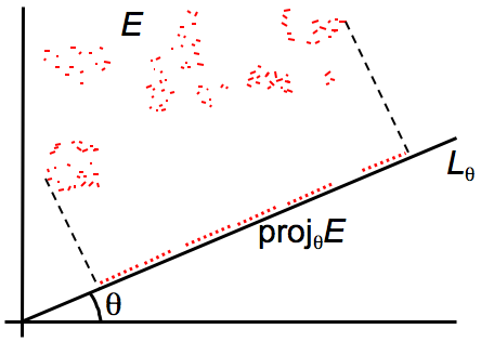
This survey paper looks back on 70 years of research about “fractal projections.” A projection is like a shadow: you take a shape in space and see what it looks like when you shine light from a direction onto a line or a plane. The paper explains a classic result (Marstrand’s projection theorem) and shows how it sparked a huge area of study. It also covers many modern advances, new techniques, and how these ideas connect to other parts of math and even number theory.
Key questions the paper explores
- If you have a fractal set (a very detailed, often self-similar shape), what happens to its “size” or “complexity” when you look at its shadow (projection) onto a line or a plane?
- Do most directions give you the same amount of detail in the shadow, or are there special directions where the shadow looks simpler?
- How do different ways of measuring “size” (Hausdorff, box-counting, packing, Assouad, Fourier dimensions) behave under projection?
- What happens if we only project in a restricted family of directions (for example, along a smooth curve of directions instead of all possible ones)?
- For special fractals built from repeated patterns (self-similar or self-affine sets), can we predict exactly how their shadows look in specific directions?
How the research works (methods explained simply)
Researchers use several mathematical tools, often with everyday analogies:
- Energy methods: Imagine spreading “electric charge” across a set and measuring how strongly points interact; this “energy” gives a way to quantify the set’s fine structure and connects to dimension.
- Fourier transforms: Think of a shape being turned into waves. Looking at how quickly these waves die out tells you about the shape’s roughness and how it behaves when projected. It’s a powerful tool from harmonic analysis.
- Probability and dynamics: Sometimes fractals come from repeated random or systematic rules. Tools from dynamical systems and ergodic theory help analyze their typical behavior.
- Discretization and additive combinatorics: Break the problem into many small, finite pieces (like pixels or tiles) and use clever counting and geometry to get bounds.
- Geometry of directions: The Grassmannian is the “space of all possible lines or planes.” Understanding volumes and dimensions of exceptional directions (where projections are atypical) involves geometry on these spaces.
Main findings and why they matter
1) The classic result (Marstrand’s projection theorem)
- In the plane (2D), if you project a set E onto a line at almost any angle, the “dimension” of the shadow equals the smaller of the set’s dimension and 1. In higher dimensions, projecting onto an m-dimensional subspace gives the smaller of the set’s dimension and m.
- If the set is “big enough” (dimension larger than the target), then the shadow has positive length/area (it’s not just a dust).
This matters because it says: for almost all directions, projections behave predictably.
2) Exceptional directions (where projections are smaller than expected)
- Most directions are fine, but some special ones can produce unusually small shadows.
- A major recent breakthrough (Ren and Wang, 2023) proved Oberlin’s conjecture, giving sharp bounds on how large the set of bad directions can be in the plane. Roughly: the bigger you force the shadow to be, the fewer bad directions there can be.
- Similar bounds exist in higher dimensions, with improvements in special cases.
Why it matters: We can now tightly control how often projections fail to be “as big as they should be,” which is crucial in analysis and geometric measure theory.
3) Other ways to measure size (dimensions) under projection
Different “dimension” notions capture different aspects; here’s how they behave:
- Box-counting dimension: Uses counts of small boxes needed to cover the set. The paper introduces “dimension profiles” and capacities (a refined way to measure complexity) that give sharp, almost-sure formulas for box-dimensions of projections.
- Packing dimension: Like an upper version of Hausdorff dimension. Many box-dimension projection results extend to packing dimension using similar profiles.
- Intermediate dimensions: A scale bridging Hausdorff (finer) and box-counting (coarser). There is a Marstrand-type theorem: almost all directions give projections whose intermediate dimensions match a corresponding profile.
- Assouad dimension: Focuses on the thickest parts of a set (worst-case local structure). It behaves very differently: there’s no general “almost sure” equality for projections, and the behavior can be wild. Still, for almost all directions, projections don’t drop below min(m, Assouad dimension of E).
- Fourier dimension: Based on how fast the Fourier transform (the “wave” representation) decays. Projections preserve some Fourier information; for special “Salem sets” (where Fourier and Hausdorff dimensions agree), projections have no exceptional directions at all.
Why it matters: These tools let you pick the right measurement for your problem and predict how projections will behave.
4) Projections in restricted direction families
- If you only look along a smooth curve of directions (instead of all directions), newer results still guarantee Marstrand-type behavior for almost all parameters on the curve, provided the curve has enough “curvature” (is non-degenerate).
- In 3D, for non-degenerate curves of directions:
- Projecting onto lines: almost all directions give dimension equal to min(original dimension, 1), and if the set is large enough, the shadow has positive length. There are sharp bounds on how many parameters can be exceptional.
- Projecting onto planes: similarly, you get min(original dimension, 2), with positive area if the set is large enough, and bounds on exceptional parameters.
Why it matters: Real-world problems often only allow certain directions; these results guarantee good behavior even under such constraints and connect to advanced topics (e.g., number theory via Diophantine approximation).
5) Special fractal sets (self-similar and self-affine)
- For fractals built from repeated scaled copies (like the Sierpiński triangle), the rotation structure matters:
- Finite rotation groups can force dimension drops in some directions (aligned shadows can “stack” in a simpler way).
- Dense rotations (e.g., rotations by irrational multiples of π) often eliminate exceptional directions entirely: all projections have the expected dimension min(original, target).
- Conditions like the open set condition help ensure dimensions are exactly what simple formulas predict.
Why it matters: Many fractals in nature and applications are self-similar/self-affine. Understanding their projections exactly—sometimes for every direction—makes the theory practical and predictive.
Implications and impact
- A unifying picture: From Marstrand’s original theorem to modern techniques, we now have powerful tools to predict and control how fractals behave under projection.
- Cross-pollination: The field draws on harmonic analysis, dynamical systems, probability, combinatorics, and geometry. Advances here have led to solutions of long-standing conjectures (Oberlin’s, Furstenberg set conjecture) and even supported progress in number theory (a quantitative version of the Oppenheim conjecture).
- Applications: Projections are central in imaging, signal processing, data analysis, and modeling complex patterns. These results guide what information survives or is lost when you only see data from certain angles or resolutions.
In short, this survey shows that the simple idea of “shadows of fractals” leads to deep mathematics, powerful methods, and surprising connections across different areas—still driving active research today.
Knowledge Gaps
Knowledge gaps, limitations, and open questions
The following list highlights concrete issues the paper indicates are missing, uncertain, or left unexplored, and where targeted research could advance the field:
- Optimal exceptional-set bounds in higher dimensions: Determine sharp Hausdorff-dimension bounds for the set of subspaces V in G(n,m) where dim proj_V(E) falls below thresholds (generalizing sharp planar results like Oberlin’s theorem to n>2 and all parameter ranges), and construct extremal examples achieving these bounds.
- Exceptional-set bounds for box and packing dimensions: Improve the current Kaufman-type and Falconer-type bounds for exceptional directions under projections (which are noted as unlikely to be sharp), and establish sharp analogues of Oberlin-type formulas for box and packing dimensions in both the plane and higher dimensions.
- Packing dimension in the plane: Clarify the sharpness of known bounds for the size of exceptional directions with small packing dimension and extend these results to Rn→G(n,m), including regimes s≥(dim_p(E)/2) and the “≤” versus “<” threshold behavior.
- Intermediate dimensions: Develop bounds for the Hausdorff/packing dimension of the exceptional set of directions where the projected upper (and lower) intermediate dimension falls below the profile value; characterize when the function θ↦overline{dim}_θ(E) is continuous at θ=0 (give necessary and sufficient conditions on E); and extend Marstrand-type results to restricted families of directions/subspaces.
- Assouad spectrum and quasi-Assouad dimension: Resolve whether Marstrand-type almost-sure projection results hold for the Assouad spectrum dim_Aθ (0<θ<1) and for the quasi-Assouad dimension; if not, characterize the nature and size of exceptional direction sets and identify minimal hypotheses under which such results can be recovered.
- Assouad projections in higher dimensions: Generalize plane results controlling exceptional directions (e.g., dim{θ: dim_A(proj_θ E) < min{1, dim_A(E)}}=0) to projections onto m-dimensional subspaces in Rn, and determine optimal bounds for the size of the exceptional set.
- Fourier dimension under projections: Establish whether a Marstrand-type theorem holds for the Fourier dimension of projections (i.e., dim_F(proj_V(E))=min{m, dim_F(E)} for almost all V) and develop sharp exceptional-set bounds informed by the Fourier spectrum; construct explicit extremal examples to test sharpness.
- Restricted direction families (curves in S2, R3→lines): Close the gap between current exceptional-set bounds (e.g., “≤ s” versus “≤ max{0,1+(s−dim(E))/2}”) by identifying the exact optimal bound; determine sharp bounds for the set of parameters t where Lebesgue measure of projections vanishes when dim_H(E)>1; and relax non-degeneracy assumptions by identifying minimal curvature conditions guaranteeing Marstrand-type conclusions.
- Projections onto planes from R3: Extend exceptional-set bounds to cover s in 1,2, and obtain sharp bounds on the parameter set where Lebesgue measure of projections is zero for sets with dim_H(E)>2; determine optimality and extremizers.
- Higher-dimensional restricted projections: Develop sharp Marstrand-type and exceptional-set results for non-degenerate submanifolds of G(n,m) in Rn (n>3), including k-parameter families (curves, surfaces) and mth-order tangent spaces, with explicit dependence on curvature and parameter dimension.
- Self-similar sets with finite rotation group: Characterize the entire set of directions producing dimension drops (size, structure, exact projection dimension as a function of direction), including quantitative bounds on the Hausdorff/packing dimension of the exceptional direction set; extend to overlapping IFS beyond OSC/SSC.
- Self-similar sets with dense rotations: Beyond Hausdorff dimension equality in all directions, determine uniform regularity of projection measures (absolute continuity, Lp bounds, smoothness) and extend to non-linear C1 mappings; quantify how overlap affects these properties.
- Self-affine attractors: Provide systematic, sharp projection-dimension results (Hausdorff, packing, box, Assouad, Fourier) for broad classes of self-affine IFS (e.g., dominated splitting, strong separation, random/self-affine carpets), including exceptional-set size and measure positivity, and identify conditions ensuring “no exceptional directions.”
- Non-Borel/analytic sets: Extend projection theory to non-measurable sets via effective dimension/computability frameworks; clarify which projection properties are independent of standard set-theoretic axioms and develop robust, axioms-insensitive formulations.
- Measures with multifractal structure: Develop unified, sharp results for the dimensions (Hausdorff, packing, Fourier, profiles) and absolute continuity of projections of dynamically defined measures, expressed in terms of entropies and Lyapunov exponents, including optimal exceptional-set bounds.
- Interior of projections: Improve and generalize thresholds guaranteeing non-empty interior of typical projections (e.g., refining E>2m conditions), and obtain sharp bounds on the exceptional set of directions with empty interior.
- Structure of exceptional direction sets: Go beyond dimension bounds to characterize geometric/topological properties (porosity, rectifiability, self-similarity, arithmetic structure) of exceptional direction sets and construct canonical extremal examples achieving known bounds.
- Computational methods: Develop practical algorithms to estimate projection dimensions and the size of exceptional sets for concrete fractals (self-similar, self-affine, random), enabling empirical validation and exploration of theoretical bounds.
Practical Applications
Immediate Applications
The following applications leverage the survey’s core results on projection theorems, exceptional sets, and dimension profiles to inform workflows and tools that can be deployed now.
- Dimension-aware imaging protocols (healthcare, materials, geoscience)
- Use Marstrand-type results and restricted-direction theorems (e.g., non-degenerate curves for line/plane projections in R³) to design scanning protocols that avoid “bad angles” and ensure that 2D projections retain positive measure and near-maximal dimension for almost all viewing directions.
- Workflow: incorporate non-degenerate directional sweeps in CT/MRI/micro-CT and SEM/tomography; include coverage planning that satisfies curvature conditions to guarantee almost-sure outcomes (Theorems for projections in non-degenerate families).
- Assumptions/dependencies: targets are well-modeled as Borel/analytic sets with fractal-like geometry; scanning trajectory meets non-degeneracy; instrument SNR/resolution adequate for dimension estimation.
- Projection risk certification for dimensionality reduction (software, data science/ML)
- Estimate box/packing dimension profiles (sE) via capacity-based kernels to quantify expected information loss when projecting to m dimensions: pick m so that mE ≈ original dimension; monitor exceptional-set size (Kaufman-/Falconer-type bounds).
- Tool: a Python/R library implementing capacity kernels φ_rs and profile estimation, reporting “projection risk” and bounds on exceptional directions.
- Assumptions/dependencies: datasets treated as compact/Borel subsets; finite-resolution effects handled via profile approximations; profiles computed over representative samples.
- Robust coverage planning in remote sensing (environmental monitoring, GIS)
- Plan satellite/airborne sensor trajectories satisfying curvature/non-degeneracy constraints so that for almost all times t, projections (e.g., line-of-sight profiles) retain dimension/minimal measure of terrain features (coastlines, forests).
- Workflow: flight path optimization with projection-exception bounds to reduce missed-feature risk; angle scheduling to increase signal detectability for fractal landscapes.
- Assumptions/dependencies: scene has nontrivial fractal structure; trajectory controllable; georegistration accuracy sufficient.
- Texture rendering and compression with projection guarantees (software, computer graphics)
- For self-similar textures with dense rotations, rely on guaranteed dimension preservation across all viewing angles; tune anisotropic filtering/mipmapping using projected dimension bounds to allocate resolution where loss is expected (finite rotation cases).
- Tool: rendering pipeline module that computes or tags texture assets by rotation group type (dense vs finite) to inform sampling rates and antialiasing.
- Assumptions/dependencies: texture assets modeled by IFS; classification of rotation group feasible; pipeline supports angle-aware filtering.
- Fractal-based material and porous media characterization (materials, energy)
- Infer 3D microstructure complexity from planar cross-sections/slices using projection dimension bounds; verify that dimension drops are within known limits (e.g., Järvenpää–Falconer–Howroyd bounds for box/packing dimensions).
- Workflow: standardized imaging + dimension estimation protocol using packing/box profiles to quantify pore network connectivity and scale invariance.
- Assumptions/dependencies: samples exhibit fractal behavior at measured scales; finite-resolution and noise accounted for in profile estimation.
- Multi-view feature robustness auditing (biometrics, forensics, computer vision)
- Use dimension bounds (packing/Assouad) to identify directions where projected complexity could drop; flag acquisition angles with potential feature-loss; prioritize “almost all” directions where features remain robust.
- Tool: acquisition planner and quality checker that recommends angles and reports dimension-preserving confidence scores.
- Assumptions/dependencies: target patterns have fractal-like signatures; capture device orientation adjustable; profiles reliably estimated from observed data.
- Education and research tooling (academia, education)
- Interactive modules demonstrating “almost all” projection phenomena, exceptional-set bounds (e.g., Oberlin’s conjecture), and dimension profiles; use to teach measure-theoretic thinking about information preservation under projection.
- Tool: web app with sliders for set dimension, projection dimension m, and kernel parameters, visualizing bounds/sharp examples.
- Assumptions/dependencies: numerical stability and sampling sufficiency for illustrative examples.
- Number theory and computational mathematics workflows (academia)
- Incorporate restricted-direction projection results (used in quantitative Oppenheim advances) to tighten constants in algorithms involving values of quadratic forms and lattice enumeration.
- Assumptions/dependencies: application domain matches curvature/non-degeneracy setups; algorithms accept improved geometric bounds.
Long-Term Applications
The following opportunities depend on further research, validation, or scaling. They build on methods like decoupling, additive combinatorics, CP processes, Fourier/energy techniques, and the newly-resolved conjectures.
- Dimension-aware autonomous sensing and exploration (robotics, defense, environmental monitoring)
- Plan sensor orientations/paths that follow non-degenerate direction curves so that the robot’s projections capture environmental complexity with high probability; dynamically adapt orientations based on estimated mE to retain detail during SLAM and mapping.
- Potential product: “dimension-preserving” planning module integrated into autonomy stacks.
- Dependencies: fast online dimension/profile estimates; robust non-degeneracy enforcement; validation in cluttered, noisy environments.
- Fractal-informed compressed sensing and sampling (communications, signal processing)
- Use Fourier dimension/spectrum and Salem-set insights to design sampling schemes (measurement matrices) tailored to signals with fractal spectral decay; aim for improved reconstruction guarantees tied to spectrum profiles.
- Potential product: compressed sensing toolkits with fractal priors and spectrum-aware recovery.
- Dependencies: empirical identification of fractal priors in real signals; theory-to-practice bridge for guarantees; algorithmic efficiency.
- Multi-view foundation models regularization (software, AI/ML)
- Regularize embeddings across views using packing/Assouad/Fourier spectra to enforce invariance of complexity under projection; mitigate “view collapse” in multimodal learning; detect angles/augmentations that cause excessive dimension drop.
- Potential tool: training regularizers that penalize dimension loss across projected embeddings.
- Dependencies: scalable dimension/spectrum estimators for high-dimensional latent spaces; theoretical guidance on generalization benefits.
- Medical imaging standards based on dimension profiles (healthcare, policy)
- Develop certification benchmarks using capacity-based box/packing profiles to assure imaging systems recover complexity under angle/projective variability; define minimal directional coverage criteria leveraging exceptional-set bounds.
- Potential product: standards and compliance tests for scanners (CT/MRI) targeting fractal pathologies (e.g., vascular/airway trees).
- Dependencies: consensus on clinical relevance of fractal metrics; standardized profile estimation methods; regulatory adoption.
- Cybersecurity anomaly detection via projection ensembles (cybersecurity)
- Build random-subspace/angle ensembles that, by exceptional-set bounds, assure anomalies with fractal signatures remain detectable across most projections; tune ensemble size using Oberlin-type bounds on bad directions.
- Potential product: “projection-safe” anomaly detectors with provable coverage rates.
- Dependencies: demonstration that target anomalies exhibit fractal behavior; integration with streaming analytics; robustness to adversarial manipulation.
- 3D reconstruction/inversion for fractal structures (materials, geoscience, archaeology)
- Use dimension-preserving projection theory to design inversion algorithms for fractal microstructures from sparse multi-angle slices; quantify uncertainty via exceptional-set bounds; apply to subsurface imaging and cultural heritage scans.
- Dependencies: robust forward models and noise-handling; sufficient angle coverage; computational scalability.
- Geospatial planning and urban analytics (policy, urban planning)
- Model street networks and built environments via fractal dimensions; use projection bounds to estimate visibility/coverage from constrained vantage lines (e.g., corridors, UAV routes); optimize surveillance, signage, or emergency egress planning.
- Dependencies: validated fractal modeling of urban forms; access to controllable vantage sets; incorporation into planning tools.
- Cryptographic and steganographic primitives from controlled projection behavior (security)
- Explore sets with tailored exceptional-direction profiles to conceal/reveal information under most projections while leaking under specific angles; utilize dense vs finite rotation group IFS behavior.
- Dependencies: rigorous security proofs; practical encodings; resilience to noise and discretization.
- Energy and porous media optimization (energy, materials)
- Use projection-based dimension constraints to design materials with desired flow/transport properties manifested in cross-sections; target microstructures with minimal dimension loss across operational viewing/sensor directions.
- Dependencies: empirical linkage between fractal dimension and transport; manufacturing control; multi-scale validation.
Cross-cutting assumptions and dependencies
- Many results assume sets are Borel/analytic and fractal-like over the observed scale range; finite-resolution and noise can bias dimension estimates.
- “Almost all directions” guarantees depend on non-degenerate parameterizations (curvature conditions) or full Grassmannian sampling; constrained settings require restricted-direction bounds.
- Capacity-based kernels and energy/Fourier integral estimates need efficient numerical approximations; scaling to large datasets requires algorithmic innovations.
- Exceptional-set bounds often provide worst-case dimension estimates rather than explicit constructive angle lists; practical systems may use randomized or coverage-based strategies to hedge against rare bad directions.
- For IFS-based applications, rotation-group properties (dense vs finite) significantly affect projection reliability; classification of assets/models may be required.
Glossary
- additive combinatorics: Area of mathematics studying combinatorial properties of addition in sets, often used in discrete and harmonic analysis. Example: "discretisation of problems and additive combinatorics"
- analytic set: A set with a descriptive set-theoretic structure ensuring measurability and regularity; commonly assumed in geometric measure theory. Example: "Let be a Borel or analytic set."
- Assouad dimension: A notion of dimension capturing the most concentrated local scaling behavior of a set; sensitive to the thickest parts. Example: "The {\it Assouad dimension} of is given by"
- Assouad spectrum: A one-parameter family refining Assouad dimension by restricting scales via a parameter, interpolating between local and global behavior. Example: "Variants on Assouad dimension include the {\it Assouad spectrum } "
- Borel set: A set generated from open sets via countable unions, intersections, and complements; the standard measurable sets in analysis. Example: "Let be a Borel or analytic set."
- box-counting dimension: Also called Minkowski dimension; defined via asymptotics of minimal covering numbers by small sets. Example: "The {\it lower} and {\it upper box-counting dimensions} of a non-empty and compact are given by"
- capacity (with kernel φ_rs): A potential-theoretic quantity associated with a set and a kernel, used to characterize box and projection dimensions. Example: "The {\it capacity} of a compact with respect to is given by"
- circular maximal function: A maximal operator over circles used in harmonic analysis to control averaging operators; applied to projection problems. Example: "Pramanik, Yang and Zahl \cite{PYZ} proved \eqref{PYZ} using a circular maximal function"
- compact manifold: A manifold that is compact as a topological space; here the parameter space of subspaces. Example: "Then is an -dimensional compact manifold"
- convolution formulae: Identities relating Fourier transforms of convolutions, central in harmonic analysis. Example: "applying Parseval's theorem and the convolution formulae to the energy expression in \eqref{endef} gives"
- CP processes: Processes (e.g., CP-chains) in ergodic theory used to analyze scaling sceneries of measures. Example: "drawing on modern techniques from ergodic theory, CP processes, Fourier transforms, discretisation of problems and additive combinatorics"
- decoupling method: A harmonic analysis technique that decomposes functions according to frequency to obtain sharp inequalities. Example: "Gan, Guth and Maldague \cite{GGM} used a decoupling method to obtain \eqref{GGM}"
- dense rotations: Property that the group generated by rotational parts of similarities is dense in the rotation group, eliminating exceptional projections. Example: "A rather different situation occurs if the IFS has {\it dense rotations}, that is the rotation group is dense in the full group of rotations "
- Diophantine approximation: Study of how well real numbers/vectors can be approximated by rationals/integers; connected here via projection results. Example: "This turns out to have applications to Diophantine approximation."
- effective dimension: An algorithmic information-theoretic notion of fractal dimension used in computability contexts. Example: "Lutz and Stull \cite{LS} have used effective dimension and computational complexity"
- energy integral (s-energy): A double integral of a kernel measuring interaction at scale s; characterizes Hausdorff dimension via finiteness. Example: "for the -{\it energy} of the measure "
- Erdős–Volkmann conjecture: Statement that no Borel subrings of ℝ have Hausdorff dimension strictly between 0 and 1. Example: "a very short proof of the Erd\H{o}s-Volkmann conjecture"
- exceptional set (of directions): The set of projection directions where a typical dimension or measure conclusion fails. Example: "the `exceptional set' of projection directions for which $\mbox{\rm proj}_\theta E < \min\{ E, 1\}$"
- Falconer-type estimate: Bounds on sizes of exceptional parameter sets that depend on how far a dimension is from a threshold. Example: "have become known as
Kaufman-type' andFalconer-type' estimates respectively." - Fourier dimension: A dimension notion defined by decay rates of Fourier transforms of measures supported on the set. Example: "Then the {\it Fourier dimension } of is given by"
- Fourier spectrum: A family of dimensions interpolating between Fourier and Hausdorff dimensions via a parameter. Example: "Fraser \cite{Fra3} introduced the {\it Fourier spectrum} of a set "
- Fourier transform: Integral transform mapping a measure/function to its frequency representation, central in projection proofs. Example: "Writing for the Fourier transform of "
- fractional Brownian motion: A family of Gaussian processes with self-similarity and long-range dependence; used in dimension results. Example: "images of sets under fractional Brownian motion \cite{KX,Xia}"
- Furstenberg set conjecture: A conjecture about the minimal dimension of sets intersecting many lines in large-dimensional slices. Example: "Oberlin \cite{Obe} noted the analogy between this conjecture and the Furstenberg set conjecture."
- Grassmanian: The space of all m-dimensional linear subspaces of ℝn, used to parameterize projection directions. Example: "we write for the Grassmanian of -dimensional subspaces of "
- Hausdorff dimension: A fundamental fractal dimension defined via Hausdorff measure; stable under Lipschitz maps. Example: "relates the Hausdorff dimension of a plane set to the dimensions of its orthogonal projections onto lines."
- high-low method: A harmonic analysis technique splitting into high/low frequency parts to prove projection bounds. Example: "proved by Gan et al \cite{GGGHMW} using the `high-low' method."
- homothety: A similarity transformation with only scaling and translation (no rotation or reflection). Example: "three homotheties (similarities without rotations) of ratio "
- invariant measure (on Grassmanian): A measure unchanged under the action of the orthogonal group; the natural measure on G(n,m). Example: "which carries a natural invariant measure "
- intermediate dimensions: A one-parameter family interpolating between Hausdorff and box dimensions via restricted cover sizes. Example: "Intermediate dimensions were introduced by Falconer, Fraser and Kempton \cite{FFK} in 2020 to interpolate between Hausdorff dimensions and box dimensions."
- iterated function system (IFS): A collection of contractions whose unique compact fixed set is the attractor. Example: "Recall that an {\it iterated function system} (IFS) is a family of contractions "
- Kaufman-type estimate: Direct upper bounds on dimensions of exceptional parameter sets, independent of excess dimension. Example: "have become known as
Kaufman-type' andFalconer-type' estimates respectively." - kernel (φ_rs): A radial function used in defining capacities/energies to study dimensions and projections. Example: "We define kernels for , by"
- Lebesgue measure: The standard measure on Euclidean space/lines; used for “almost all” statements and positivity of projections. Example: "we will write for Lebesgue measure on any line "
- Lipschitz map: A map with bounded distortion of distances; ensures Hausdorff dimension does not increase. Example: "Since orthogonal projection is a Lipschitz map that does not increase distances between points"
- local dimensions (of measures): Pointwise scaling exponents of a measure; relate to Hausdorff/packing dimensions of measures. Example: "Lower and upper Hausdorff and packing dimensions of measures can be defined in terms of local dimensions"
- Lyapunov exponents: Exponential rates of divergence in dynamical systems; relate to dimensions of invariant measures and their projections. Example: "the dimension of projected measures can be expressed in terms of entropies and Lyapunov exponents."
- Marstrand's projection theorem: A foundational result giving almost-sure dimension and measure of projections of sets. Example: "Marstrand's projection theorem in the plane \cite{Mar} may be stated as follows."
- Marstrand-type theorem: Any result asserting that a dimension property holds for almost all parameters (e.g., directions). Example: "we say that a `Marstrand-type theorem holds'."
- non-degenerate (curve of directions): A curve whose direction, velocity, and acceleration span ℝ3, ensuring curvature for restricted projections. Example: "We say that the curve of directions is {\it non-degenerate} if"
- open set condition (OSC): A separation condition for IFSs requiring a disjoint open set mapped into itself by the maps. Example: "the {\it open set condition} (OSC) if there is a non-empty open set such that with this union disjoint"
- Oppenheim conjecture: A statement about values of indefinite quadratic forms at integers being dense, with quantitative refinements. Example: "The Oppenheim conjecture, formulated by Alex Oppenheim in 1929 and originally proved by Margulis \cite{Marg} in 1987"
- orthogonal projection: Projection onto a subspace along perpendicular directions; central to projection theorems. Example: "write for orthogonal projection onto "
- orthonormal map: A rotation or reflection; the linear part of a similarity. Example: "where is the contraction ratio, is an orthonormal map, i.e. a rotation or reflection"
- packing dimension: A dual to Hausdorff dimension defined via packing measures; often larger than Hausdorff dimension. Example: "Packing measures and packing dimension were introduced by Tricot \cite{Tri} in 1982"
- Parseval's theorem: Identity equating L2 norms of a function and its Fourier transform; used to relate energy integrals and decay. Example: "applying Parseval's theorem and the convolution formulae to the energy expression in \eqref{endef} gives"
- potential theory: The study of harmonic functions and energies; provides tools (energies, capacities) for dimension estimates. Example: "Kaufman \cite{Kau} gave a new proof of Theorem \ref{marthm}(i) using potential theory"
- quasi-Assouad dimension: A limit of the Assouad spectrum as the parameter approaches 1, capturing near-local scaling. Example: "and the related {\it quasi-Assouad dimension } which may be expressed as"
- restricted directions (projections): Studying projections only along a lower-dimensional family of directions instead of all subspaces. Example: "Projections in restricted directions"
- rotation group (of an IFS): The group generated by the rotational parts of similarities in an IFS; its structure controls projection behavior. Example: "The {\it rotation group} "
- Salem set: A set whose Fourier dimension equals its Hausdorff dimension, implying optimal projection behavior. Example: "In particular, if is a {\it Salem set}, that is if "
- self-similar set: The attractor of an IFS of similarities; exhibits exact scaled copies of itself. Example: "the attractor is termed {\it self-similar}."
- similarity dimension: The value s solving Σ r_is = 1 for an IFS of similarities; equals the set’s dimension under separation. Example: "similarity dimension , then $\mbox{\rm proj}_V E<s$ for some "
- strong open set condition (SOSC): A strengthening of OSC requiring the open set to intersect the attractor. Example: "and the {\it strong open set condition} (SOSC) if such a can be chosen so ."
- strong separation condition (SSC): A strict separation condition requiring the basic pieces in the IFS union to be disjoint. Example: "An IFS of similarities ... satisfies the {\it strong separation condition} (SSC) if the union (\ref{attractor}) is disjoint"
- tangent space (mth order): A higher-order generalization of tangent directions used in advanced projection theorems in higher dimensions. Example: "the projection of to the th order tangent space of at "
- upper semi-continuous (function): A function whose superlevel sets are closed; used in constructing sets with prescribed Assouad projection behavior. Example: "for any upper semi-continuous "
- unit sphere : The 2-dimensional sphere in ℝ3, parameterizing directions for line/plane projections in 3D. Example: " (the 2-sphere embedded in )"
Collections
Sign up for free to add this paper to one or more collections.