Deep Learning for Financial Time Series: A Large-Scale Benchmark of Risk-Adjusted Performance
Abstract: We present a large scale benchmark of modern deep learning architectures for a financial time series prediction and position sizing task, with a primary focus on Sharpe ratio optimization. Evaluating linear models, recurrent networks, transformer based architectures, state space models, and recent sequence representation approaches, we assess out of sample performance on a daily futures dataset spanning commodities, equity indices, bonds, and FX spanning 2010 to 2025. Our evaluation goes beyond average returns and includes statistical significance, downside and tail risk measures, breakeven transaction cost analysis, robustness to random seed selection, and computational efficiency. We find that models explicitly designed to learn rich temporal representations consistently outperform linear benchmarks and generic deep learning models, which often lead the ranking in standard time series benchmarks. Hybrid models such as VSN with LSTM, a combination of Variable Selection Networks (VSN) and LSTMs, achieves the highest overall Sharpe ratio, while VSN with xLSTM and LSTM with PatchTST exhibit superior downside adjusted characteristics. xLSTM demonstrates the largest breakeven transaction cost buffer, indicating improved robustness to trading frictions.
Paper Prompts
Sign up for free to create and run prompts on this paper using GPT-5.
Top Community Prompts
Explain it Like I'm 14
What is this paper about?
This paper tests many modern AI models to see which ones are best at turning noisy financial data into trading signals that make steady, risk-aware profits. The authors focus on “risk-adjusted” performance, especially a score called the Sharpe ratio, which rewards higher returns but penalizes bumpy, risky ups and downs.
In short: they compare lots of deep learning models on 15 years of daily market data (2010–2025) to find out which ones make the most reliable trading decisions across many kinds of markets (commodities, stock indexes, bonds, and currencies).
The main questions the researchers asked
- Which kinds of models are best at reading financial time series (numbers that change over time, like prices) and producing good trading signals?
- Do fancy, general-purpose AI models (like Transformers) work well in finance, or do models designed to handle time and noise work better?
- How stable are the results over different market periods (calm years vs. wild years)?
- How do trading costs (paying a “fee” each time you change your position) affect the profits?
- Are the results robust, meaning they don’t depend on lucky random starts or special settings?
How did they do the study?
The data
They used daily information from futures markets across:
- Commodities (like metals or agriculture),
- Energy,
- Stock indexes,
- Government bonds,
- Currencies (FX).
Futures are standardized contracts that bet on the future price of something. The data covered 2010–2025, including calm and turbulent periods. Financial data is hard: it’s noisy (lots of randomness), patterns are weak, and what worked last year might not work this year.
The models they tested
They compared simple and advanced approaches. Here’s a plain-English guide:
- Linear models (like simple rules): fast and simple, but not very flexible.
- Recurrent neural networks (RNNs), especially LSTMs and xLSTMs: these have “memory,” so they can remember patterns over time.
- Transformers and patch-based Transformers (like PatchTST): models that look across the whole sequence at once; patching means grouping days together to smooth noise.
- State-space models (like Mamba/Mamba2): models that keep a compact “summary” of the past, designed to handle long sequences efficiently.
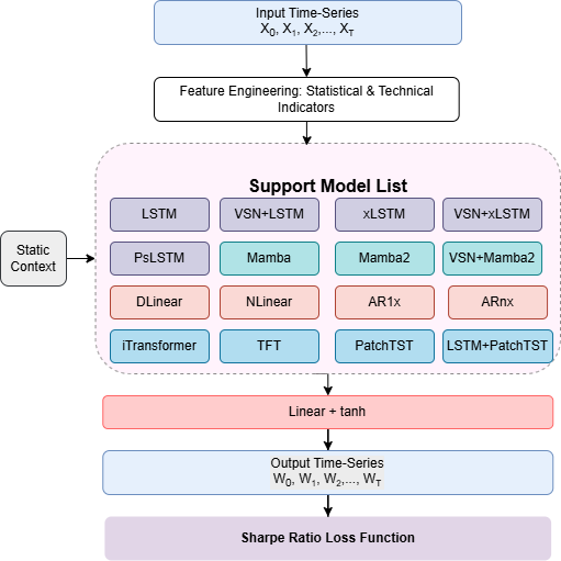
- Hybrids (like VSN+LSTM, LSTM+PatchTST, VSN+xLSTM): combinations that first pick the most useful features (using a Variable Selection Network, or VSN) and then apply a strong time-learning model.
A useful analogy:
- Think of the data as a long, messy song.
- Linear models are like using a single, straight beat to follow the rhythm.
- LSTMs are like musicians with good memory, remembering earlier themes.
- Transformers listen to many parts of the song at once.
- State-space models keep a neat notebook summary of what’s happened.
- VSN is like a volume knob that turns down noisy instruments and turns up the helpful ones.
How the trading signals worked
- Each model looks at a window of past days and outputs a signal between -1 and +1.
- +1 means “go fully long” (bet the price will go up).
- -1 means “go fully short” (bet the price will go down).
- They used “volatility targeting,” which is like cruise control for risk: if a market is very jumpy, the position size is reduced; if it’s calmer, it can be larger. This keeps overall risk more consistent.
- They trained models to directly maximize the Sharpe ratio, not just to predict tomorrow’s price. The Sharpe ratio is like “points per risk”: higher is better if you can get returns without too much shakiness.
How they judged the models
They went beyond simple average returns. They looked at:
- Sharpe ratio and statistical tests (to check if results are real, not luck),
- Downside risk (how bad the worst stretches were),
- Tail risk (how bad rare, extreme losses could be),
- Turnover and transaction costs (how much trading you do and how much that would cost),
- Robustness (do results hold across different years and random starting points?),
- Speed/efficiency (how heavy the models are to run).
They also checked “breakeven transaction cost,” which is the highest trading fee you could pay before the model’s profits disappear. Think of it as: how much “friction” can this strategy handle and still make money?
What did they find?
- Models that are built to handle time well and reduce noise consistently beat simple linear models and many general-purpose deep models.
- The best results came from hybrids that first select useful features and then use strong time-memory tools.
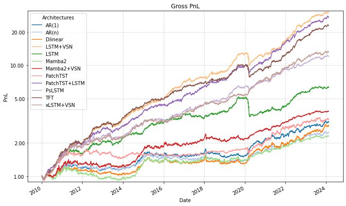
- VSN + LSTM (often called VLSTM) had the highest overall Sharpe ratio across 2010–2025.
- LSTM + PatchTST and VSN + xLSTM also did very well, especially on downside risk (they handled bad times better).
- xLSTM had the largest “breakeven transaction cost,” meaning it was more resilient to trading fees and frequent rebalancing.
- Linear models sometimes did okay in certain years (especially very volatile ones) but were not reliable over the whole period.
- Generic Transformers and some state-space models weren’t consistently strong in this financial setting. In finance, the signal is weak and noisy, so models that can selectively remember and filter noise have an edge.
- Results stayed strong even when the team reduced the number of random runs (“seeds”), which suggests the findings are robust, not just due to lucky training runs.
Why this matters: it shows that in finance, where real patterns are faint and change over time, architecture choices that highlight useful signals and store them wisely are key.
Why it matters and what could happen next
- For researchers and practitioners: If you want steadier, risk-aware trading performance, favor models that:
- Select important features (VSN),
- Keep adaptive, long-term memory (LSTM/xLSTM),
- Smooth out noise (patching or preprocessing),
- And train directly on what you ultimately care about (risk-adjusted returns like the Sharpe ratio).
- For real-world trading: xLSTM’s stronger buffer against transaction costs hints it could be more practical when fees and slippage matter, while VLSTM’s high Sharpe suggests strong overall “quality” of signals.
- For future work: The study used a particular dataset and setup. Testing on other markets, different time scales (like hourly or minute data), and changing cost assumptions would help confirm how universal these findings are.
In one sentence: The paper shows that smart “memory-and-selection” deep learning models, trained to optimize steady returns rather than pure prediction accuracy, can make more robust trading decisions in the noisy world of finance.
Knowledge Gaps
Knowledge gaps, limitations, and open questions
The paper provides a broad benchmark, but several aspects remain uncertain or unexplored. Future work could address the following gaps:
- External validity limited to a single vendor’s cross-asset futures/FX dataset at daily frequency (2010–2025); no tests on other markets (e.g., single stocks, options), regions, or intraday data to assess portability.
- Universe construction and survivorship bias are not fully specified (e.g., inclusion rules, handling of delistings/contract switches); sensitivity to alternative continuous-contract methodologies (ratio vs. difference back-adjustment, front-month selection rules) is not examined.
- Feature scope appears confined to price-based statistical/technical indicators; the incremental value of exogenous information (macro, carry/roll/premium signals, COT positioning, fundamentals, alternative data) is not evaluated.
- No comparison to strong finance baselines (e.g., canonical time-series momentum, carry, or simple trend-following rules with the same volatility targeting), leaving the incremental alpha over standard rule-based strategies unclear.
- Portfolio construction is effectively per-asset with scalar signals, equal risk allocation, and no cross-asset optimization; benefits of multi-output models that jointly consider covariance, sector structure, or cross-asset lead–lag effects are not assessed.
- Training objective optimizes a pooled sample Sharpe using batch-aggregated returns; sensitivity to objective design (per-asset vs. pooled objectives) and comparisons to alternative differentiable risk objectives (Sortino, CVaR, drawdown penalties, utility-based losses) are missing.
- Transaction costs are set to
c_k=0during training and primary evaluation; only post-hoc, constant per-asset breakeven costs are reported. Realistic, time-varying execution frictions (bid–ask spreads, slippage, market impact, fees), capacity limits, and net performance under plausible cost models are not analyzed. - High turnover (often ~700–1000 annualized) raises questions about feasibility under liquidity, tick size, and lot-size constraints; capacity/scalability by asset and the trade-off between turnover and performance are not quantified.
- Execution assumptions (signal at close, trade effective next bar) are not stress-tested against close-to-open execution, overnight gaps, limit moves, or partial fills; latency and slippage sensitivity remain unmeasured.
- Volatility targeting is fixed at 10% using EWMA; the dependence of results on target volatility, EWMA decay, and alternative risk estimators (e.g., GARCH, realized vol) is not explored.
- Statistical inference reports HAC t-stats but does not correct for multiple model comparisons or seed selection (no SPA/Reality Check/DM tests); uncertainty around model ranking and the probability of outperformance is not quantified with bootstraps or confidence intervals.
- Seed selection ensembles the top
Sseeds by validation loss (from 50 or 25 runs), introducing selection bias; the single-seed performance distribution and deployable variance are not fully characterized. - Hyperparameter fairness and tuning parity across architectures are under-specified (lookback
L, hidden sizeH, depth, patch length, parameter counts, learning rates, early stopping); negative results for transformers/SSMs may reflect suboptimal tuning rather than inherent limits. - Compute efficiency is discussed qualitatively, but training time, memory footprint, and energy cost per model are not reported; practical deployability at scale is unclear.
- Model- and component-level ablations are limited: the incremental contributions of VSN, LSTM denoising, patching, ticker embeddings, and other architectural choices are not isolated in controlled experiments.
- SSM implementation choices (e.g., static HiPPO transitions without horizon jitter) are restrictive; performance of alternative SSMs (S4/DSS/GSS, adaptive horizons, diagonal/low-rank variants) and their tuning space remain unexplored.
- Non-stationarity handling is implicit; there are no explicit tests for regime-change robustness (e.g., covariate shift diagnostics, rolling re-tuning cadence comparisons, pre-registered forward-only tests with frozen hyperparameters).
- Interpretability is not pursued: feature/ticker importances from VSN, temporal saliency, or factor attribution (exposure to trend, carry, equity/bond betas) are not analyzed; economic plausibility of learned patterns remains opaque.
- Sensitivity analyses are sparse: key design choices (lookback window
L, patch length, tanh output bounds, EWMA λ, target volatility) and their effects on both performance and turnover are not reported. - Cross-sectional dependence is not explicitly modeled (beyond shared parameters and embeddings); whether attention across assets or covariance-aware decoders improves performance is an open question.
- Robustness to data quality issues (missing values, roll date conventions, calendar mismatches, holidays) and preprocessing choices (standardization windows, de-meaning) is not evaluated.
- Risk and financing frictions (futures margining, collateral returns, exchange/clearing fees, funding costs) are omitted; whether rankings persist under realistic financing environments is unknown.
- Generalization across horizons and tasks is untested (only one-step-ahead daily signals); multi-horizon forecasting, event-conditioned strategies, and alternative targets (directional accuracy, volatility forecasting) are left open.
- Reproducibility is limited: code is “available upon request,” and several implementation specifics (exact architecture configs, training schedules, rolling window lengths, evaluation splits) are not exhaustively documented for independent replication.
- Comparisons to strong non-deep ML baselines (e.g., gradient Boosted Trees, random forests, regularized linear models with engineered features) are absent; the necessity of deep architectures versus shallow, interpretable models is not established.
- Training stability and regularization (gradient variance under Sharpe loss, weight decay, dropout, early stopping criteria) are not reported; convergence behavior and failure modes under different seeds are unclear.
Practical Applications
Practical Applications of “Deep Learning for Financial Time Series: A Large-Scale Benchmark of Risk-Adjusted Performance”
Below are concrete, real-world applications derived from the paper’s findings, methods, and innovations. They are grouped into Immediate Applications and Long-Term Applications. Each item notes sectors, examples of tools/products/workflows, and key assumptions/dependencies affecting feasibility.
Immediate Applications
These can be deployed now with realistic effort in professional and academic environments.
- Sharpe-optimized signal engines for cross-asset futures trading
- Sectors: Finance (buy-side quant, CTAs/managed futures, prop trading)
- Tools/workflows: Adopt VLSTM, LPatchTST, or xLSTM as core signal generators; implement the modular pipeline (feature extraction → sequence model → tanh projection → volatility targeting); train via negative Sharpe loss with pooled-batch Sharpe as per DeePM; deploy daily EOD rebalancing.
- Assumptions/dependencies: Availability of high-quality continuous futures data (2010–2025 analogues), adequate compute for training/seed ensembling, risk controls for position bounds and leverage, awareness that results are conditional on daily data and this backtesting protocol; training ignores transaction costs (gross), so turnover management is critical in production.
- Turnover-aware instrument selection using breakeven transaction cost (c*) screening
- Sectors: Finance (portfolio managers, execution desks)
- Tools/workflows: Post-hoc c* computation per asset to filter or size allocations; prioritize assets/contracts with higher c* buffers; pair with turnover dashboards and seed-ensemble position smoothing.
- Assumptions/dependencies: Stationarity of turnover patterns and liquidity; realistic mapping from c* to live costs; scalability limits in illiquid contracts (e.g., Lumber, Oats, Milk III).
- Robust signal ensembling to improve stability and reduce trading frictions
- Sectors: Finance (quant research, systematic trading), Software (platforms for quant MLOps)
- Tools/workflows: Train multiple seeds, select top S by validation Sharpe, average signals to lower variance and turnover; integrate with CI/CD pipelines for research-to-production promotion.
- Assumptions/dependencies: Sufficient compute budget for multi-seed training; monitoring for overfitting in seed selection; governance to prevent “seed mining.”
- Regime-robust backtesting and reporting standards
- Sectors: Finance (risk, validation), Policy (regulatory guidelines), Academia (methodology pedagogy)
- Tools/workflows: Standardize reports including HAC-adjusted t-stats, subperiod Sharpe, downside/tail metrics (MaxDD, Calmar, CVaR), and passive-relative diagnostics; include seed-robustness experiments as part of model approval.
- Assumptions/dependencies: Organizational buy-in to extend backtesting templates; data coverage across multiple regimes (e.g., post-GFC, 2020 volatility).
- Upgrades to momentum/trend-following systems with hybrid recurrent + patching
- Sectors: Finance (managed futures, multi-asset)
- Tools/workflows: Replace traditional time-series momentum rules with LPatchTST or VLSTM-based signals; retain volatility targeting and risk budgets; evaluate strategy overlays on existing CTA stacks.
- Assumptions/dependencies: Consistency of performance when mapped to live execution; realistic slippage and carry/roll adjustments; position scaling under [-1, 1] bounds may need modification.
- Academic benchmarking and curriculum modules for low-SNR time series
- Sectors: Academia (ML for finance), Education
- Tools/workflows: Use the paper’s architecture suite (linear, RNN, transformer, SSM, hybrids) and evaluation protocol to teach pitfalls of generic benchmarks; assign Sharpe-optimized training labs; encourage ticker embeddings and feature selection (VSN) for asset-specific learning.
- Assumptions/dependencies: Access to similar datasets (or public proxies), code access (available upon request), compute in teaching labs.
- Buy-side quant research workflow templates emphasizing inductive bias
- Sectors: Finance (quant R&D), Software (internal libraries)
- Tools/workflows: Template repositories implementing VLSTM/xLSTM/LPatchTST with ticker embeddings, volatility targeting, and pooled Sharpe loss; comparison harness across regimes; ablation frameworks for inductive bias (feature selection vs. attention vs. recurrence).
- Assumptions/dependencies: Team familiarity with PyTorch/JAX; data engineering for EOD features; integration with existing backtesting engines.
- Risk dashboards prioritizing tail behavior and downside robustness
- Sectors: Finance (risk management, product oversight), Investor relations
- Tools/workflows: Integrate worst-3m Sharpe, min-annual Sharpe, CVaR(5%), and Calmar into live dashboards; flag strategy behavior in volatile regimes; compare LSTM variants vs. hybrids on risk-adjusted basis.
- Assumptions/dependencies: Histories long enough to compute stable tail estimates; regular recalibration under regime shifts.
- Sell-side/fintech analytics products for model diagnostics
- Sectors: Finance (sell-side research, data vendors), Software
- Tools/workflows: Offer “Sharpe-optimized model checkups” that score client strategies against benchmark architectures; provide turnover vs. performance frontiers and c* estimates; produce per-asset alpha maps.
- Assumptions/dependencies: Client data sharing and confidentiality; clear disclaimers on generalization beyond backtests.
- Corporate treasury and asset–liability overlays for hedging programs
- Sectors: Corporate finance (treasury), Commodities/FX hedgers
- Tools/workflows: Use xLSTM/VLSTM-derived signals as overlays for timing hedge ratios (reduce/increase hedge when signals are strong/weak) with strict risk controls; focus on liquid instruments with favorable c*.
- Assumptions/dependencies: Strict governance and limits; careful mapping from speculative signals to hedging objectives; conservative turnover targets.
Long-Term Applications
These require further research, scaling, or development before broad deployment.
- Differentiable transaction-cost–aware training and multi-objective optimization
- Sectors: Finance (systematic trading, execution research), Software (AutoML for finance)
- Tools/workflows: Extend loss to include differentiable proxies for turnover/slippage; jointly optimize Sharpe, drawdown, and CVaR; adaptively penalize turnover by asset liquidity.
- Assumptions/dependencies: Reliable cost models and differentiable approximations; robust execution–signal feedback loops; nonstationary cost regimes.
- Real-time and intraday extensions with microstructure features
- Sectors: Finance (intraday/short-horizon trading), Market making
- Tools/workflows: Adapt VLSTM/xLSTM/LPatchTST to intraday bars or LOB features; handle non-synchronous multi-asset data; latency-aware deployment.
- Assumptions/dependencies: High-frequency data infrastructure; strict latency and reliability constraints; risk of strategy crowding.
- Foundation models and representation learning for financial sequences
- Sectors: Finance (platform research groups), Academia (time-series foundation work), Software (model hubs)
- Tools/workflows: Pretrain hybrid recurrent models (VSN+LSTM/xLSTM) on large multi-asset, multi-frequency corpora; fine-tune for specific tasks (trend-following, mean reversion, risk forecasting); explore few-shot generalization (building on X-Trend lineage).
- Assumptions/dependencies: Large-scale curated datasets and compute; prevention of data leakage and survivorship bias; stability under regime shifts.
- Cross-domain applications in energy, commodities, and supply chain risk
- Sectors: Energy/utilities, Commodity trading/hedging, Manufacturing procurement
- Tools/workflows: Apply patching + recurrence architectures to forecast/hedge exposures (e.g., fuels, power, FX); integrate with procurement schedules and storage constraints; optimize hedge timing akin to portfolio weights.
- Assumptions/dependencies: Domain-specific features (weather, load, shipment data); reliable mapping from forecasts to actionable hedges; operational constraints.
- AI model governance frameworks for capital markets
- Sectors: Policy/regulation, Financial compliance and model risk management (MRM)
- Tools/workflows: Codify requirements for seed-robustness tests, subperiod reporting, HAC statistics, and c* analysis; develop standardized disclosures for risk-adjusted optimization and turnover profiles.
- Assumptions/dependencies: Regulatory consensus and industry adoption; clarity on how Sharpe-optimized training interacts with investor suitability and risk disclosures.
- AutoML for low-SNR time-series with inductive bias search
- Sectors: Software (quant platforms), Finance (research tooling), Academia
- Tools/workflows: Automated pipeline that searches across inductive biases (feature selection, patching, recurrence, state-space) and tunes objective trade-offs; delivers ready-to-validate candidates with risk reports.
- Assumptions/dependencies: Guardrails to prevent overfitting/data snooping; computational budgets; reproducibility and audit trails.
- Adaptive portfolio construction beyond tanh-limited scalar signals
- Sectors: Finance (multi-asset portfolio management), Insurance (ALM), Endowments
- Tools/workflows: Move from scalar signals and simple volatility targeting to multi-output position vectors with constraints, dynamic risk budgets, and cross-asset interactions; integrate with optimizer layers.
- Assumptions/dependencies: Differentiable optimizers with constraints; robust estimation of cross-asset covariance; interpretable allocation logic for committees.
- Stress-testing frameworks driven by learned regime embeddings
- Sectors: Finance (risk), Policy (macroprudential oversight)
- Tools/workflows: Use model states/ticker embeddings to infer regime labels; replay performance under synthetic shocks; assess model sensitivity to volatility clusters and heavy tails.
- Assumptions/dependencies: Stable mapping from latent states to interpretable regimes; methods to generate plausible shocks; validation data for tail events.
- Retail and advisory integration via simplified, low-turnover variants
- Sectors: Wealth management, Robo-advisors
- Tools/workflows: Distill xLSTM-based signals into low-turnover ETF overlays; client-specific risk targets; periodic (e.g., monthly) rebalancing with turnover caps.
- Assumptions/dependencies: Reduced-complexity models that retain efficacy; clear explanations for clients; alignment with suitability and fee structures.
- Cross-asset corporate exposure management and dynamic hedging assistants
- Sectors: Corporate treasury, Airlines/shipping, Agri-business
- Tools/workflows: Assist treasurers with dynamic hedge ratio recommendations informed by low-SNR–oriented models; integrate forecasts with cashflow calendars and risk limits.
- Assumptions/dependencies: Accurate exposure measurement; governance for model overrides; robust backtesting against business KPIs.
- Open, standardized benchmark suite for low-SNR time series
- Sectors: Academia, Open-source software, Industry consortia
- Tools/workflows: Public datasets and code (when license permits), standardized metrics (Sharpe, HAC t-stats, downside), and established baselines (linear, RNN, transformer, hybrid) to evaluate new methods beyond seasonal, high-SNR benchmarks.
- Assumptions/dependencies: Data licensing, reproducibility across institutions, community maintenance.
Notes on feasibility across items:
- Many immediate applications depend on robust data pipelines (clean continuous futures, feature engineering), compute for training/ensembling, and risk/compliance processes.
- The paper’s results are explicitly conditional on daily, cross-asset futures (2010–2025), zero-cost training (gross), volatility targeting at 10%, and the authors’ backtesting choices; generalization to other markets, frequencies, and cost regimes requires revalidation.
- Hybrid architectures with strong inductive bias (e.g., VSN+LSTM, LPatchTST, xLSTM) showed the best balance of performance, stability, and turnover—making them priority candidates for near-term adoption.
Glossary
- AR1x: A per-feature autoregressive model of order 1 used as a minimal temporal benchmark in time-series forecasting. "The AR1x model \cite{ar1} serves as a minimal temporal benchmark, capturing short-term autocorrelation in returns."
- AR(n)x: A per-feature autoregressive model of order n serving as a linear baseline in the study. "linear specifications such as AR1x, ARx, DLinear, and NLinear occasionally achieve strong single-year Sharpe ratios"
- Back-adjusted (ratio-adjusted backwards) methodology: A procedure for constructing continuous futures contracts by adjusting for roll-induced jumps. "using a ratio-adjusted backwards methodology (i.e., back-adjusted to remove roll-induced price jumps)"
- Basis points: A unit equal to one hundredth of a percent (0.01%), commonly used to express transaction costs or yields. "The tables report annualised, volatility-rescaled gross and net returns together with annualised turnover and the implied breakeven transaction cost in basis points."
- Breakeven transaction cost: The maximum constant trading friction a strategy can bear before its cumulative profit becomes zero. "we conduct a post-hoc, asset-level breakeven transaction cost analysis"
- Breakeven transaction cost buffer: The margin by which a strategy’s performance can absorb transaction costs before profits vanish. "xLSTM demonstrates the largest breakeven transaction cost buffer, indicating improved robustness to trading frictions."
- CAGR (Compound Annual Growth Rate): The rate of return that would produce the observed cumulative growth if profits were compounded annually. "presenting compound annual growth rates (CAGR)~\cite{elton_mpt}"
- Calmar ratio: A performance metric defined as annualized return divided by maximum drawdown. "including maximum drawdown (Max DD), Calmar ratio (Calmar), worst three-month Sharpe ratio (Worst 3m Sharpe), minimum annual Sharpe ratio (Min Ann. Sharpe), and 5\% conditional value at risk (CVaR 5\%)."
- Conditional Value at Risk (CVaR 5%): The expected loss beyond the 5% worst-case loss threshold. "including maximum drawdown (Max DD), Calmar ratio (Calmar), worst three-month Sharpe ratio (Worst 3m Sharpe), minimum annual Sharpe ratio (Min Ann. Sharpe), and 5\% conditional value at risk (CVaR 5\%)."
- DeePM framework (regime-robust): A training approach computing objectives over pooled returns to better proxy out-of-sample Sharpe. "Following the regime-robust DeePM framework \cite{deepm_regime_robust}, we compute the Sharpe ratio objective on pooled portfolio returns concatenating all sequences in the batch"
- EWMA (Exponentially Weighted Moving Average): A volatility estimator that weights recent observations more heavily than older ones. "We estimate the ex-ante conditional volatility for each asset using an Exponentially Weighted Moving Average (EWMA) estimator"
- Ex-ante conditional volatility: The model’s forecast of future volatility based on recent data and a specific estimator. "We estimate the ex-ante conditional volatility for each asset using an Exponentially Weighted Moving Average (EWMA) estimator"
- FX: Foreign exchange markets or instruments. "foreign-exchange (FX) futures"
- HAC (heteroskedasticity and autocorrelation consistent) t-statistics: Inference statistics robust to time-varying variance and serial correlation. "heteroskedasticity and autocorrelation consistent -statistics ( HAC)~\cite{newey_west}"
- Heavy-tailed return distributions: Return distributions with higher probability of extreme values than Gaussian. "including heavy-tailed return distributions, volatility clustering, and strong deviations from Gaussianity."
- HiPPO (High-order Polynomial Projection Operators): A class of operators that maintain compressed summaries of past information in evolving models. "HiPPO (High-order Polynomial Projection Operators) matrices \cite{hippo}, which maintain compressed representations of past information as the model evolves."
- Hit rate (Pesaran–Timmermann): The proportion of correct directional predictions, often evaluated with the Pesaran–Timmermann test. "hit rate (Hit)~\cite{pesaran_timmermann}"
- Hyperbolic tangent activation: A bounded activation function mapping inputs to [-1, 1], used to constrain trading signals. "followed by a hyperbolic tangent () activation function to bound the output"
- Information ratio: Excess return relative to a benchmark divided by tracking error. "the information ratio (Info. Ratio), HAC -statistic relative to passive ( HAC v Passive), and correlation with passive returns (Corr. v Passive)"
- iTransformer: An architecture that applies attention across features instead of time, viewing each feature as a token. "The inverted Transformer \cite{itransformer} applies attention across feature dimensions rather than time, treating each feature as a token."
- Leverage factor: A scaling term derived from volatility estimates to equalize risk across assets. "This estimation induces a time-varying leverage factor, defined as $\text{vs\_factor}_{t,k} = \frac{1}{\sigma_{t,k}$, which dynamically scales position sizes in response to shifting market regimes."
- Linear-attention-like behavior: Attention computations with linear complexity in sequence length, improving scalability. "Mamba2 \cite{mamba2} claims to achieve a mathematically principled architecture with linear-attention-like behavior \cite{lin_attn} while supporting arbitrarily large lookback windows."
- Lookback window: The fixed number of past timesteps used as input for forecasting. "Given a fixed lookback window of length "
- LPatchTST: A hybrid architecture combining LSTM-based denoising with PatchTST’s patch-based attention. "LSTM + PatchTST (LPatchTST). This architecture combines explicit recurrence with attention by using an LSTM as a channel-wise temporal denoiser prior to PatchTST."
- Mamba: A selective state-space model with implicit temporal recurrence and linear-time complexity. "Mamba models \cite{mamba, mamba2} belong to the class of selective state-space models (SSMs)~\ref{appdx:mamba}, which maintain a latent state that is updated recursively over time."
- Mamba2: A refined Mamba variant with simplified state transitions and increased head dimensionality for stability and speed. "Mamba2 refines this formulation by simplifying the state transition structure and increasing head dimensionality, leading to improved numerical stability and throughput."
- Maximum drawdown: The largest peak-to-trough decline experienced by a strategy. "including maximum drawdown (Max DD), Calmar ratio (Calmar), worst three-month Sharpe ratio (Worst 3m Sharpe)"
- NLinear: A non-recurrent linear model operating on normalized inputs, used as a time-series baseline. "DLinear and NLinear \cite{nlinear} are non-recurrent linear models that apply learned linear mappings to fixed-length input windows."
- PatchTST: A transformer that processes sequences as temporal patches to improve robustness and receptive field. "PatchTST \cite{patchtst} segments the input sequence into temporal patches, which are embedded and processed via self-attention."
- PnL (Profit and Loss): The cumulative or per-period monetary gains or losses of a strategy. "before its cumulative PnL is driven to zero."
- Projection head: The final module mapping hidden representations to scalar outputs or signals. "The second stage is a unified projection head applied to the terminal hidden state ."
- PsLSTM: A patch-based sLSTM variant combining patching with exponential-gated recurrence for noise robustness. "Patch sLSTM \cite{pslstm} integrates the patching strategy of PatchTST with the recurrent inductive bias of sLSTM."
- Regime (market regime): Distinct market conditions or periods with differing dynamics (e.g., volatility or trends). "across time and economic regimes"
- Rolling windows (training): A training procedure that iteratively updates models using consecutive windows of data. "All models are trained using rolling windows and evaluated in a fully out-of-sample trading framework."
- Sharpe ratio: Risk-adjusted performance metric defined as mean return divided by return volatility. "The loss function is defined as the negative differentiable annualized Sharpe Ratio"
- Sharpe-ratio optimization: Directly optimizing model parameters to maximize Sharpe rather than minimize prediction error. "with a primary focus on Sharpe-ratio optimization."
- Signal-to-noise ratio: The relative strength of the predictive signal compared to noise in the data. "These datasets exhibit strong seasonality and a high signal-to-noise ratio, in contrast to financial time series"
- sLSTM: Scalar-memory xLSTM variant using normalized exponential gates for long-range retention. "xLSTM comprises two variants: scalar LSTM (sLSTM), which maintains a scalar memory state updated via normalized exponential gates"
- State Space Models (SSMs): Models that maintain and update latent states over time to capture sequence dynamics. "belong to the class of selective state-space models (SSMs)~\ref{appdx:mamba}, which maintain a latent state that is updated recursively over time."
- TFT (Temporal Fusion Transformer): A model integrating gated recurrence, attention, and variable selection for robust forecasting. "TFT \cite{tft} integrates gated recurrent layers with interpretable attention mechanisms."
- Ticker embeddings: Learned representations for asset identifiers to enable per-asset conditioning. "We added ticker embeddings to all the models to enhance the learning per individual ticker/asset~\cite{entity_embeddings}."
- Turnover: The amount of portfolio rebalancing over time, often measured in notional units or as xGMV. "turnover, turnover as a multiple of gross market value (xGMV)~\cite{vol_target}"
- Variable Selection Networks (VSN): Modules that perform dynamic, feature-wise soft selection and embedding of covariates. "Variable Selection Networks (VSNs)~\ref{appdx:vsn}, inspired by the Temporal Fusion Transformer, are used to perform feature-wise nonlinear embedding and dynamic soft selection of relevant covariates at each time step."
- Volatility clustering: The empirical tendency for high-volatility periods to cluster over time. "including heavy-tailed return distributions, volatility clustering, and strong deviations from Gaussianity."
- Volatility targeting: Scaling positions to equalize risk contributions by targeting a specified portfolio volatility. "we employ a volatility targeting framework to equalize risk contributions across the universe~\cite{tsmom,vol_target,enhancing_tsmom}."
- Volatility-rescaled gross PnL: Profit and loss scaled to a target volatility level for comparability across strategies. "Performance comparison across models 10\% volatility-rescaled gross PnL."
- VLSTM: A hybrid of VSN and LSTM used to build compact temporal representations for financial forecasting. "VLSTM combines a VSN with an LSTM encoder to construct a compact temporal state representation."
- VxLSTM: A hybrid where VSN-selected features feed into an xLSTM with matrix-valued memory. "VSN + xLSTM (VxLSTM). In this hybrid, VSN-selected representations are directly fed into an xLSTM."
- Worst three-month Sharpe: The lowest Sharpe ratio measured over any three-month interval. "including maximum drawdown (Max DD), Calmar ratio (Calmar), worst three-month Sharpe ratio (Worst 3m Sharpe)"
- xGMV (turnover as a multiple of gross market value): Turnover normalized by gross market value, indicating trading intensity relative to portfolio size. "turnover as a multiple of gross market value (xGMV)~\cite{vol_target}"
- xLSTM: An LSTM variant with exponential gating and memory normalization, enabling improved long-range retention via matrix-valued memory. "xLSTM replaces LSTM’s traditional sigmoid gating with exponential gating and a normalization term, while also employing a memory matrix rather than a scalar value."
Collections
Sign up for free to add this paper to one or more collections.