Linear equivalence of nonlinear recurrent neural networks
Abstract: Large nonlinear recurrent neural networks with random couplings generate high-dimensional, potentially chaotic activity whose structure is of interest in neuroscience, machine learning, ecology, and other fields. A fundamental object encoding the collective structure of this activity is the $N \times N$ covariance matrix. Prior analytical work on the covariance matrix has been limited to low-dimensional summary statistics, not the full high-dimensional object for a specific realization of the couplings. Recent work proposed an ansatz in which, at large $N$, the covariance matrix for a typical quenched realization takes the same form as that of a linear network with the same couplings, driven by independent noise, with mean-field order parameters setting the effective transfer function and the noise spectrum. Here, we derive this ansatz using the two-site cavity method, providing two distinct derivations that offer complementary perspectives. The first decomposes each unit's activity into a linear component and a nonlinear residual, and shows that cross-covariances between residuals at distinct sites are strongly suppressed, so that residuals act as independent noise within a linear network. The second writes a self-consistent matrix equation for the covariance matrix. A naive Gaussian closure for the joint statistics of activity at distinct sites gives the wrong equation; the cavity method separates Gaussian and non-Gaussian contributions, which enter at the same order, and produces the correct one. We verify the predictions numerically across a range of network sizes. These results extend linear equivalence from feedforward high-dimensional nonlinear systems, where the weights being analyzed are independent of their inputs, to recurrent networks, where the activities depend on the same couplings that generate them.

Paper Prompts
Sign up for free to create and run prompts on this paper using GPT-5.
Top Community Prompts
Explain it Like I'm 14
What is this paper about?
This paper studies very large, randomly wired brain-like networks where each unit (think “neuron”) constantly influences the others. Even though each unit behaves in a nonlinear way (like a dimmer that saturates rather than a simple volume knob), the authors show that one important summary of the network’s activity—the covariance matrix, which tells you which units tend to fluctuate together—can be predicted as if the whole network were linear. In simple terms: for big enough networks, a complicated nonlinear system “looks” linear when you focus on how pairs of units co-vary over time.
What questions are they asking?
- Can we compute the full covariance matrix of a large nonlinear recurrent network (not just averages) for a typical random wiring?
- Does this covariance matrix match the one from a linear network that has the same connections but is driven by a certain kind of “effective” noise?
- How accurate is this “linear equivalence,” and why should it hold?
How did they study it? (Methods in everyday language)
First, some simple ideas:
- Recurrent network: Every unit talks to many others, and signals loop around. This can create rich, even chaotic, activity.
- Covariance matrix: Imagine watching a crowd dance. The diagonal entries say how much each person wiggles on their own; the off-diagonal entries say how much two different people tend to move together. That full “who-moves-with-whom” map is the covariance matrix.
- Big networks simplify: When there are many random connections, certain averages become predictable. This is the spirit of “mean-field” ideas: focus on typical behavior in the crowd rather than tracking every detail.
What they actually did:
- Mean-field order parameters: They used standard tools (called dynamical mean-field theory) that summarize “typical” single-unit behavior in large random networks. These give two key quantities: how a unit tends to respond to inputs on average, and how wiggly its activity is over time.
- Two-site cavity method: To understand relationships between two different units, they temporarily “remove” those two units from the network, study the rest (which is simpler), then add the two back and track how signals flow to and from them. This lets them carefully separate different effects, including subtle feedback loops.
Two complementary derivations:
- Linear + residual split
- Think of each unit’s activity as “linear response to its input” plus a leftover “residual” that captures the nonlinear part.
- The authors prove that, across different units, those nonlinear leftovers barely line up with each other (their cross-covariances are very small). So those leftovers behave like independent noise driving a linear system.
- Result: The full covariance matrix equals the one you’d get from a linear network with the same wiring, driven by independent noise whose strength is set by the mean-field quantities.
- Self-consistent matrix equation
- They write an equation that the covariance matrix must satisfy.
- If you naïvely pretend the inputs to different units are jointly Gaussian, you get the wrong equation. The two-site cavity method fixes this by keeping both Gaussian and non-Gaussian contributions that matter at the same size.
- Solving the corrected equation gives exactly the same “linear-equivalent” covariance formula.
They also run long computer simulations to check the math, confirming how closely the linear prediction matches the real nonlinear network as the network gets bigger.
What did they find, and why does it matter?
Main findings:
- Linear equivalence: For a large nonlinear recurrent network with random connections, the entire covariance matrix is (to high precision) the same as that of a linear network with the same connections, driven by independent noise whose size is set by the mean-field theory.
- Accuracy:
- Diagonal entries (each unit’s own variability) are off by about 1/√N, where N is the number of units.
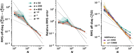
- Off-diagonal entries (pairwise co-variation) naturally shrink like 1/√N as N grows, and the linear prediction gets them right up to an even smaller error, about 1/N.
- This means the eigenvalue spectrum (the “shape” of population variability used in dimensionality reduction) is also matched in the large-network limit.
- Response matrix too: A similar “linear-equivalent” formula holds for how the network, as a whole, responds to external inputs.
Why it matters:
- This bridges a gap between linear and nonlinear worlds. For linear networks, we already have powerful tools (like random matrix theory) to compute the covariance and its spectrum exactly. The paper shows those tools can accurately describe complicated nonlinear, even chaotic, recurrent networks—if you plug in the right mean-field parameters.
- It applies directly to neuroscience (understanding large-scale neural recordings), machine learning (reservoir computing and recurrent neural networks), and ecology (multi-species interaction models), where high-dimensional, random, recurrent systems are common.
What could this lead to?
- Easier analysis and design: Engineers and scientists can analyze complex recurrent systems using well-understood linear math, as long as they estimate the mean-field parameters correctly. This can simplify predicting the dimensionality and structure of population activity, which is central to interpreting brain recordings and designing recurrent AI systems.
- Understanding learning: Since this gives a clean baseline for “untrained” random networks, it can help us see how training or plasticity reshapes collective activity.
- Broader impact: The approach suggests that many high-dimensional nonlinear systems might be “linearly equivalent” for second-order statistics (covariances), making them much easier to study and understand.
In short, the paper shows that when you look at how a huge, messy, nonlinear network’s parts move together, the network behaves almost exactly like a linear system—once you choose the right effective “gain” and “noise.” This makes a hard problem much simpler without losing important information about collective behavior.
Knowledge Gaps
Knowledge gaps, limitations, and open questions
Below is a single, focused list of unresolved issues and limitations suggested by the paper that future work could address:
- Connectivity structure beyond i.i.d.: Extend the derivations to non-i.i.d. couplings, including low-rank perturbations, block-structured (multi-population) matrices, Dale’s law (E/I sign constraints), and motifs; determine how the linear-equivalent form and resolvent change.
- Partial or full symmetry: Develop an analogue of the equivalence under correlated pairs , where Onsager reaction terms appear; derive the correct covariance equation and quantify deviations from the i.i.d. asymmetric case.
- Sparse networks: Establish whether the linear-equivalent covariance holds for sparse graphs (e.g., or degree) and identify the appropriate scaling and corrections to the cavity arguments.
- Heavy-tailed couplings: Analyze couplings with infinite-variance (e.g., Lévy) distributions and quantify if/when Gaussian local-field approximations and Price/Furutsu–Novikov steps remain valid or require replacement.
- Correlated external drive across units: Generalize the ansatz to input processes with nontrivial cross-unit covariance (common or structured noise), and derive the modified matrix formulas and conditions for off-diagonal residual suppression.
- Near-critical behavior: Quantify how the element-wise error scales as , when the resolvent norm can grow; provide explicit bounds on the precision as a function of distance to instability.
- Finite-size, non-asymptotic guarantees: Replace and RMS statements with high-probability, constant-explicit bounds over the coupling ensemble, and characterize the distribution (not just RMS) of entry-wise errors.
- Nonstationary dynamics: Extend the equivalence to time-varying or transient regimes (time-dependent statistics, switching, learning-induced nonstationarity) where stationarity and time-translation invariance are absent.
- Broader nonlinear single-unit models: Provide full derivations (not just plausibility) for the bistable-unit, Hebbian-plasticity, and generalized Lotka–Volterra examples; specify assumptions on (e.g., causality, Lipschitz constants) under which the equivalence holds.
- Discrete-time and delay/synaptic-filter networks: Generalize to discrete-time RNNs and to couplings with temporal kernels or delays; derive the frequency-domain resolvent and assess if the residual-noise interpretation survives.
- Spiking/point-process models: Investigate whether analogous linear equivalence holds for spiking networks (e.g., LIF with conductance or current noise) and identify the right effective transfer/response and noise spectra.
- Higher-order statistics: Determine whether a comparable linear-equivalent approximation exists for third- and fourth-order cross-cumulants and other nonlinear observables beyond the covariance.
- Full distribution of cross-covariances: Go beyond RMS suppression to characterize the pairwise cross-covariance distribution (tails, dependence on network modes/eigenvectors) and its finite- deviations.
- Robustness to structured perturbations: Quantify how small low-rank or modular perturbations to produce spectral “spikes” and modify the covariance; derive a rank- corrected ansatz and its random-matrix predictions.
- Error-control mechanisms: Provide a systematic $1/N$ expansion (TAP-like corrections) for both the response and covariance matrices, identifying the leading correction terms beyond the current leading-order result.
- Identifiability and inverse problems: Develop and analyze procedures that use the ansatz to infer spectral properties (or components) of from empirical and estimated , including stability and sensitivity to sampling noise.
- Sampling effects: Incorporate finite-time sampling noise into the theory; derive confidence intervals or bias corrections for estimated covariance spectra when validating the ansatz empirically.
- Universality with respect to nonlinearity: Specify the minimal regularity and smoothness conditions on (or ) under which residual cross-covariances are ; identify counterexamples (e.g., nonsmooth or strongly saturating regimes).
- Multistability and non-ergodicity: Assess whether the equivalence holds within individual attractors in multistable regimes, and how it depends on initial-condition mixtures or slow switching between attractors.
- Comprehensive numerical map: Systematically test the precision across , , nonlinearities, coupling distributions, and input statistics; quantify the needed to reach target error levels as a function of frequency and proximity to criticality.
- Explicit spectral predictions: Provide closed-form eigenvalue densities for for commonly used nonlinearities and parameter ranges, beyond the references to prior numerical/analytical spectra.
- Relation to fluctuation–response structure: Clarify when fluctuation–dissipation-like relations fail or approximately hold in these nonequilibrium networks, and whether the linear-equivalent framework yields useful approximations linking and .
- Heterogeneity in gains/time constants: Extend the ansatz to units with heterogeneous single-unit parameters (gains, time constants), and derive the resulting block- or diagonal-weighted resolvent form.
- Frequency-resolved error control: Provide frequency-dependent error bounds that account for the shape of and , especially in high- and low-frequency limits.
Practical Applications
Overview
This paper proves a “linear equivalence” for large nonlinear recurrent networks with i.i.d. asymmetric couplings: the full, quenched covariance matrix of a nonlinear RNN in its stationary regime is, with controlled error, equal to that of a linear network with the same couplings, a scalar effective transfer function S(ω), and an effective noise spectrum C(ω). It also provides a leading-order approximation for the full response matrix. The result is constructive and computable: one can replace long nonlinear simulations with matrix resolvents M(ω) = (I − S(ω)J)⁻¹ and use random matrix theory to analyze spectra.
Below are practical applications that follow from these findings and methods. Each item lists likely sectors, candidate tools/products/workflows, and key assumptions/dependencies that impact feasibility.
Immediate Applications
These applications can be deployed now with existing theory and tooling, assuming the stated conditions are met.
- Fast, scalable characterization of covariance structure in random RNNs
- Sectors: software/ML (reservoir computing, echo state networks), neuroscience
- What: Replace expensive nonlinear simulations with closed-form/resolvent computations of covariance matrices and eigenvalue spectra using the linear-equivalent formula C̄(ω) = CΔ(ω) M(ω)M(ω)† with S(ω), CΔ(ω) from DMFT.
- Tools/workflows: Python/R/Julia packages to compute S(ω), CΔ(ω) via single-site DMFT and form M(ω); plug into existing random-matrix toolkits for spectrum/dimensionality; CI tests that compare simulation to analytic spectra.
- Assumptions/dependencies: Large N; i.i.d., asymmetric J with variance g²/N; stationary regime; spectral radius g|S(ω)| < 1; external drives stationary; typical quenched draws; off-diagonal errors are O(1/N), diagonals O(1/√N).
- Design and tuning of reservoirs via spectral targets
- Sectors: ML/software (reservoir computing), neuromorphic hardware
- What: Use the analytic link between J’s spectrum, S(ω), and covariance eigenvalues to set g, nonlinearity, and timescales to achieve target dimensionality and correlation structures before training readouts.
- Tools/workflows: Auto-tuning routines that search over g and nonlinearity parameters to match desired spectral density; dashboards for memory capacity vs. dimensionality trade-offs.
- Assumptions/dependencies: Same as above; reservoir weights are i.i.d. (or close); objectives depend primarily on second-order statistics.
- Rapid power analysis and recording-time planning for weak cross-covariances
- Sectors: neuroscience (systems/computational), experimental design
- What: Off-diagonal covariances scale as 1/√N with O(1/N) prediction error. Use this to determine sample length needed to resolve cross-covariances/eigenvalues with confidence, reducing trial-and-error.
- Tools/workflows: Experimental planning calculators that take N, g, S(ω) and output required recording durations for PCA/eigen-spectrum estimation; pre-registration guidelines.
- Assumptions/dependencies: Stationary spontaneous activity; random-like connectivity dominates; measurement noise accounted for separately.
- Benchmarking and QC for random RNN implementations
- Sectors: ML ops, hardware validation (analog/photonic/neuromorphic)
- What: Compare measured covariance spectra from hardware/simulators to linear-equivalent predictions to detect fabrication biases, drift, or unintended structure.
- Tools/workflows: Golden-spectrum tests in test suites; alerting when spectral radius/eigenvalue bulk deviates from theory beyond error bars.
- Assumptions/dependencies: Devices approximate i.i.d. random couplings; stationarity; sufficient N and SNR.
- Fast sensitivity and influence-path analysis using the response matrix
- Sectors: control/robotics (high-dim controllers), ML interpretability
- What: Use S̄φ(ω) ≈ S(ω)M(ω) to compute how inputs propagate through the network without perturbation experiments, enabling frequency-dependent gain/phase analyses.
- Tools/workflows: Frequency response modules integrating S̄φ(ω) for controller tuning; diagnostic plots of input-output gain per node.
- Assumptions/dependencies: Large N; same i.i.d. and stationarity assumptions; stable resolvent (g|S(ω)|<1).
- Dimensionality and PCA-spectrum analytics for population activity
- Sectors: neuroscience data analysis, ML diagnostics
- What: Predict participation ratio and full covariance eigenvalue spectra to interpret population recordings or model states; distinguish random-like dynamics from structured computation.
- Tools/workflows: Pipelines computing predicted spectra from fitted g and S(ω), overlaying with empirical spectra; goodness-of-fit metrics for “random vs structured” model selection.
- Assumptions/dependencies: Recording covers a random-like population; preprocessing yields stationary segments; sufficient N/time samples.
- Synthetic data generation with guaranteed second-order statistics
- Sectors: ML (simulation, privacy-preserving sharing), education
- What: Generate linear surrogates that match second-order statistics of chaotic nonlinear networks for benchmarking and teaching, avoiding costly simulations.
- Tools/workflows: Data generators that sample from linear-equivalent dynamics using M(ω) and CΔ(ω); curriculum materials demonstrating linear equivalence.
- Assumptions/dependencies: Downstream tasks depend primarily on second-order structure; users accept linear surrogates for benchmarking.
- Anomaly detection for learned/structured connectivity
- Sectors: ML model diagnostics, neuroscience (learning-induced structure)
- What: Deviations between empirical covariance and linear-equivalent predictions flag emergence of low-rank or structured connectivity after training or plasticity.
- Tools/workflows: Residual-spectrum monitors during training; tests that attribute excess outliers in eigen-spectrum to emerging structure.
- Assumptions/dependencies: Baseline untrained/random phase obeys assumptions; changes are moderate enough to detect via second-order deviations.
Long-Term Applications
These require further research and/or engineering—e.g., relaxing assumptions (non-i.i.d. J, spiking models), scaling to finite-N edge cases, or integrating into products.
- Extending linear equivalence beyond i.i.d. to structured or trained RNNs
- Sectors: ML (RNN/LSTM/GRU/Transformer-inspired RNNs), neuroscience (low-rank motifs), control
- What: Generalize to low-rank + random, block-structured, or trained couplings to obtain closed-form covariance/response with outliers and bulk (e.g., random-plus-rank-k models).
- Tools/products: Design tools that prescribe rank-k structure to sculpt targeted covariance eigenmodes; theory-backed regularizers enforcing spectral constraints during training.
- Dependencies: New theory (cavity/DMFT with structured disorder); validation on realistic tasks; potential Onsager terms for symmetric/correlated J.
- System identification: inferring effective coupling strength and transfer from data
- Sectors: neuroscience (effective connectivity), finance/markets (agent-based), ecology
- What: Invert the spectrum to estimate g and S(ω) from observed covariance, enabling regime classification (e.g., distance to chaos) and model-based compression.
- Tools/products: Estimators that fit DMFT order parameters to empirical spectra; uncertainty quantification for finite N and observation noise.
- Dependencies: Robust inverse-mapping under noise; identifiability in multi-parameter settings; stationarity.
- Controller and estimator co-design using linear-equivalent statistics
- Sectors: robotics, industrial control, signal processing
- What: Use S̄φ(ω) and C̄(ω) as priors in LQG/Kalman-style design for systems driven by high-dimensional nonlinear internal dynamics, improving robustness.
- Tools/products: Toolkits that plug linear-equivalent second-order models into control design loops; certification modules assessing stability margins via g|S(ω)|.
- Dependencies: Applicability when dynamics are dominated by internal random reservoirs; integration with plant models; safety certification.
- Accelerated training and compression via covariance-preserving surrogates
- Sectors: ML efficiency, on-device AI
- What: Distill nonlinear RNN modules into linear filters plus noise that preserve second-order behavior for tasks relying on correlations (e.g., kernel-like readouts), reducing compute/memory.
- Tools/products: Pruners/quantizers that target second-order equivalence; hybrid architectures swapping nonlinear cores for linear-equivalent blocks in inference pipelines.
- Dependencies: Task performance must hinge on second-order statistics; extension to non-stationary inputs; managing mismatch in higher-order moments.
- Enhanced analysis of spiking and biologically detailed networks
- Sectors: computational neuroscience, neuroengineering
- What: Adapt the method to spiking neuron models and networks with synaptic dynamics to predict population covariance spectra and response without brute-force simulations.
- Tools/products: Analysis suites for large spiking networks providing spectral predictions; experiment-theory matching for cortical recordings.
- Dependencies: New DMFT for spiking with effective S(ω); handling refractoriness/non-Gaussian drives; validation on data.
- Risk and resilience assessment in complex interacting-agent systems
- Sectors: finance (market microstructure), ecology (multi-species), epidemiology
- What: Use linear-equivalent covariance and response to assess amplification modes and collective fluctuations (eigenmodes) in generalized Lotka–Volterra or agent-based models.
- Tools/products: Early-warning indicators from eigenvalue bulks/outliers; scenario simulators replacing nonlinear cores with linear-equivalent statistics.
- Dependencies: Model alignment with i.i.d.-like interaction assumptions; stationarity; domain-specific constraints (e.g., positivity in ecology).
- Experimental and clinical translation for brain-computer interfaces (BCI)
- Sectors: healthcare (BCI, neuroprosthetics)
- What: Use predicted covariance/response spectra to design decoders that align with dominant population modes and to plan recording channel counts/durations.
- Tools/products: Decoder-initialization schemes based on predicted PCA spectra; adaptive recording strategies maximizing information per unit time.
- Dependencies: Stability and stationarity in clinical settings; mapping random-network priors to patient-specific physiology.
- Curriculum and standardized benchmarks for high-dimensional dynamics
- Sectors: education, research infrastructure
- What: Create curricular modules and benchmark suites leveraging the equivalence to teach DMFT/RMT and to standardize evaluation of high-dimensional dynamical models.
- Tools/products: Interactive notebooks, standardized datasets with ground-truth spectra, competitions around spectrum-matching and identification.
- Dependencies: Community adoption; maintenance of reference implementations.
Notes on Assumptions and Practical Boundaries
- Core assumptions: large N; i.i.d., asymmetric couplings with variance g²/N; stationary state; typical quenched realization; external drives stationary; g|S(ω)| < 1 to ensure resolvent exists.
- Precision: diagonal entries predicted to O(1/√N); off-diagonals to O(1/N); eigenvalue densities match in the large-N limit.
- When to be cautious: low N; significant coupling structure (low-rank, symmetry, correlations); strong non-stationarities; tasks dependent on higher-order moments beyond covariance.
- Extensions: The paper outlines how related models (e.g., networks with self-coupling, Hebbian plasticity absorbed into single-unit dynamics, generalized Lotka–Volterra) fit the same analytical scaffolding, suggesting paths to broaden applicability with further work.
Glossary
- Ansatz: A proposed form or assumption about a solution structure used to guide analysis. "Specifically, the ansatz states that at large and for a typical realization of the i.i.d.\ couplings, the covariance matrix of the nonlinear network takes the same form as that of a linear network with the same couplings, driven by independent noise, with the DMFT order parameters setting the effective transfer function and the noise spectrum."
- Causal functional: A mapping from an input history to an output that depends only on past inputs, not future ones. "The single-unit dynamics are defined by a causal functional ,"
- Cavity field: The input signal to a “removed” (cavity) unit generated by the rest of the network, treated as an external Gaussian drive. "The cavity fields are the inputs the cavity units would receive from the unperturbed reservoir."
- Cross-covariance: The covariance between signals at two different units (or times), measuring shared fluctuations. "and shows that cross-covariances between residuals at distinct sites are strongly suppressed,"
- Dynamical mean-field theory (DMFT): A large-scale analytical framework that reduces high-dimensional disordered dynamics to self-consistent single-site statistics. "For nonlinear networks, dynamical mean-field theory (DMFT)~\cite{sompolinsky1988chaos} provides scalar order parameters characterizing single-site statistics."
- Eigenvalue spectrum: The distribution of eigenvalues of a matrix, often characterizing variance modes or stability. "For linear networks, the covariance matrix can be written in closed form using simple linear algebra, and its full eigenvalue spectrum follows from random matrix theory~\cite{hu2022spectrum}."
- Four-point function: A higher-order correlation function involving products of two covariances, capturing variability of cross-covariances. "Using this construction followed by a disorder average over , they obtained self-consistent equations for the four-point function"
- Frobenius norm: A matrix norm equal to the square root of the sum of squares of all entries; akin to the Euclidean norm for matrices. "In both cases, we control the Frobenius norm of the error matrices to establish the desired RMS precision for off-diagonal entries."
- Furutsu–Novikov theorem: A result giving averages of products of Gaussian processes and functionals of them, used to relate inputs and responses. "We will repeatedly use the fact that, since is Gaussian, the Furutsu--Novikov theorem (Appendix~\ref{app:price}) gives the cross-covariance between the local field and the activity in terms of the response:"
- Gaussian closure: An approximation replacing true joint statistics with Gaussian ones (matching moments), often inaccurate when non-Gaussian contributions matter. "A naive Gaussian closure for the joint statistics of local fields at distinct sites gives the wrong equation;"
- Generalized Lotka–Volterra: A stochastic, high-dimensional model for interacting species’ abundances with random couplings. "With i.i.d.\ interspecies interactions as specified below, this becomes the generalized Lotka--Volterra model~\cite{roy2019numerical}."
- Hebbian plasticity: A learning rule where connections strengthen with co-activity of units. "Hebbian plasticity. \citet{clark2024theory} added Hebbian modifications to the couplings around quenched weights, giving total couplings , with ."
- Hermitian: A matrix equal to its conjugate transpose; implies real eigenvalues. "The property implies that is Hermitian for each : ."
- Hoffman–Wielandt inequality: A bound on how much eigenvalues can change under perturbations of a matrix. "noting that the Hoffman--Wielandt inequality bounds the mean squared distance between the ordered eigenvalue sequences by $\frac{1}{N}\|\bm{\mathcal{E}(\omega)\|_F^2 = O{\frac{1}{N}$."
- i.i.d. (independent and identically distributed): Random variables with the same distribution and independent realizations. "Throughout this paper, we consider the simplest instantiation, i.i.d.\ couplings with first and second moments"
- Local field: The total recurrent input to a unit from the network (plus possibly external drive). "where is the local field at unit "
- Onsager reaction term: A correction accounting for feedback of a unit’s activity through the network back onto itself. "producing an Onsager reaction term that introduces a nonlinear self-coupling with a convolutional kernel proportional to ~\cite{marti2018correlations,clark2023dimension}."
- Operator norm: The largest singular value of a matrix; induced 2-norm measuring maximum amplification. "the submultiplicativity of the Frobenius norm with respect to the operator norm,"
- Order parameter: A macroscopic quantity summarizing typical behavior (e.g., average variance or response) in the large-system limit. "The covariance and response matrices each have a scalar order parameter,"
- Participation ratio: A measure of effective dimensionality based on the moments of eigenvalues. "determines the effective dimensionality of neural population activity through the participation ratio \cite{gao2017theory, litwin2017optimal}."
- Path integral: A functional integral formalism used to analyze stochastic dynamics and fluctuations. "Subsequently, \citet{clark2025connectivity} obtained the same result from fluctuations around the saddle point of a path integral."
- Quenched disorder: Random parameters fixed over time (e.g., couplings) that shape dynamics but do not fluctuate dynamically. "In all of these settings, the couplings play the role of quenched disorder."
- Quenched realization: A specific fixed draw of the random couplings from the disorder ensemble. "for a typical quenched realization of the couplings."
- Random matrix theory: The study of matrices with random entries, providing spectral laws for large systems. "and the eigenvalue spectrum is accessible via random matrix theory~\cite{hu2022spectrum}."
- Resolvent: The inverse operator or its analog, used to solve linear systems and analyze spectra. "this can be solved using the resolvent (Eq.~\eqref{eq:resolvent}):"
- Response matrix: The matrix of linear responses of each unit to perturbations at every other unit across time/frequency. "Using these functional derivatives, we define the response matrix, with elements given by a stationary-state average"
- Reverberation kernel: A kernel capturing indirect interactions mediated by recurrent propagation through the network. "The reverberation kernel captures the indirect interaction: cavity unit perturbs the reservoir via , the perturbation propagates via , and the result is read out by cavity unit via ."
- Self-averaging: The property that macroscopic observables converge to deterministic values as system size grows. "are self-averaging: they become deterministic as "
- Self-consistency condition: An equation requiring that quantities computed from an assumed distribution match the assumed quantities themselves. "These order parameters are determined by a single-site self-consistency condition."
- Stationary state: A statistical state where distributions (e.g., moments) do not change over time. "We assume throughout that the network reaches a stationary state in which the activities fluctuate."
- TAP equations: Self-consistent equations (Thouless–Anderson–Palmer) for mean magnetizations in spin glasses, analogous to network self-consistency. "This situation is analogous to the TAP equations for spin glasses~\cite{thouless1977solution, plefka1982convergence},"
- Transfer function: The frequency-domain input-output mapping of a (linearized) unit or system. "with the DMFT order parameters setting the effective transfer function and the noise spectrum."
- Two-site cavity method: A cavity approach tracking the joint statistics of two units to capture non-Gaussian and finite-size effects. "We give two derivations, both rooted in the two-site cavity method~\cite{clark2023dimension}, which provides access to the joint statistics of activity at a pair of units within the network."
Collections
Sign up for free to add this paper to one or more collections.