Conditional Diffusion Sampling
Abstract: Sampling from unnormalized multimodal distributions with limited density evaluations remains a fundamental challenge in machine learning and natural sciences. Successful approaches construct a bridge between a tractable reference and the target distribution. Parallel Tempering (PT) serves as the gold standard, while recent diffusion-based approaches offer a continuous alternative at the cost of neural training. In this work, we introduce Conditional Diffusion Sampling (CDS), a framework that combines these two paradigms. To this end, we derive Conditional Interpolants, a class of stochastic processes whose transport dynamics are governed by an exact, closed-form stochastic differential equation (SDE), requiring no neural approximation. Although these dynamics require sampling from a non-trivial initialization distribution, we show both theoretically and empirically that the cost of this initialization diminishes for sufficiently short diffusion times. CDS leverages this by a two-stage procedure: (1) PT is used to efficiently sample the initial distribution, and then (2) samples are transported via the transport SDE. This combination couples the robust global exploration of PT with efficient local transport. Experiments suggest that CDS has the potential to achieve a superior trade-off between sample quality and density evaluation cost compared to state-of-the-art samplers.
Paper Prompts
Sign up for free to create and run prompts on this paper using GPT-5.
Top Community Prompts
Explain it Like I'm 14
What this paper is about (big picture)
The paper introduces a new way to draw random examples (samples) from very complicated probability shapes—think of landscapes with many separate hills and valleys—when each “check” of how good a location is (a density evaluation) is expensive. Their method is called Conditional Diffusion Sampling (CDS). It blends two ideas:
- Parallel Tempering (PT): a proven way to explore many distant hills (modes) without getting stuck.
- Diffusion-style transport: a smooth, math-guided way to move samples from an easy place to the hard target, without training any neural networks.
The goal is to get high‑quality samples while spending as few expensive checks (density evaluations) as possible.
What questions the paper asks
In simple terms, the paper asks:
- Can we build a sampler that:
- Works well on tough, multi‑peaked distributions?
- Needs no neural network training?
- Uses fewer expensive target evaluations?
- Can we design a smooth path that safely carries samples from an easy distribution to the target—and write down the moving rule exactly, not approximately?
- Can we combine PT (great at global exploration) with exact diffusion (great at local, guided transport) to beat current methods on both quality and cost?
How the method works (in everyday language)
Here’s the core idea, step by step.
- Start with two probability distributions:
- A simple “reference” distribution you can sample from easily (like a standard bell curve).
- A hard “target” distribution with multiple peaks (the one you actually want samples from).
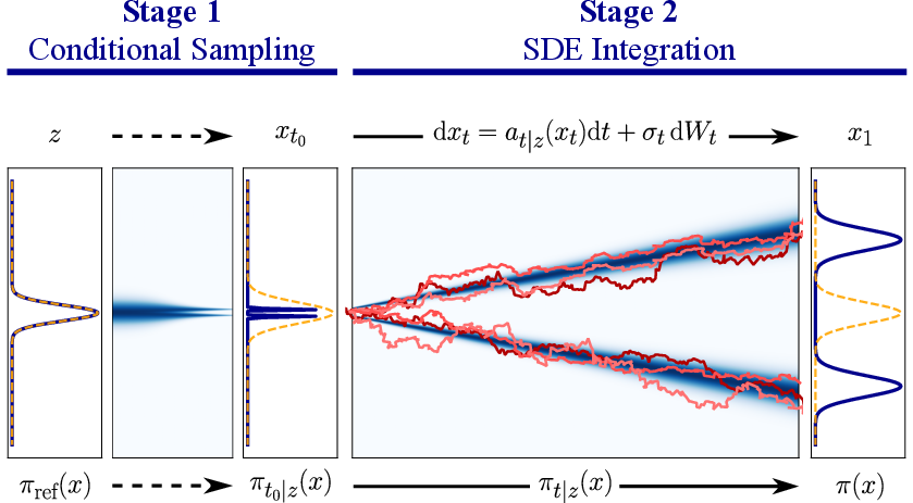
- Pick a random anchor point z from the easy reference. Now imagine every true target sample x sliding toward z over a “time” t from 1 down to 0. This creates a family of in-between distributions—when t is small, everything is clustered near z; when t is large, you get the real target.
- The authors show there’s an exact rule (a stochastic differential equation, or SDE) that tells you how to move points along this path. Importantly, this rule uses the slope of the log-density (a “score”) of the in-between distribution, and they can compute this slope exactly from the target—no neural networks needed.
- CDS runs in two stages:
- Stage 1 (Conditional Sampling): Use Parallel Tempering to sample from one of those in-between distributions at a small time t0. Because this in-between distribution is tightly clustered around z (so it overlaps the easy reference a lot), PT can move around and communicate between modes more efficiently than if it targeted the full, hard distribution.
- Stage 2 (SDE Transport): Starting from those samples, follow the exact diffusion rule from t0 to 1 to “transport” them to the true target. This step also gently corrects errors along the way, keeping samples on track.
Analogy: Imagine crossing a river. Stage 1 finds a good stepping stone near your side (easy and safe to reach). Stage 2 is like a moving walkway that carefully carries you across the river to the far bank (the target), adjusting your path as you go.
Key technical terms translated:
- Multimodal: The distribution has multiple separate “hot spots” where samples are likely.
- Density evaluation: Asking “how likely is this point?”—this can be expensive in physics or big machine learning models.
- Score (gradient of log-density): A vector that points you uphill toward higher probability; the method can compute it exactly for the in-between distributions.
- SDE (stochastic differential equation): A rule for moving with both drift (guided motion) and noise (randomness), like a particle pushed by wind and jitter.
What they found and why it matters
Main results:
- CDS achieves a better balance between sample quality and cost (number of density evaluations) than strong competitors in many tests.
- It works without any neural network training.
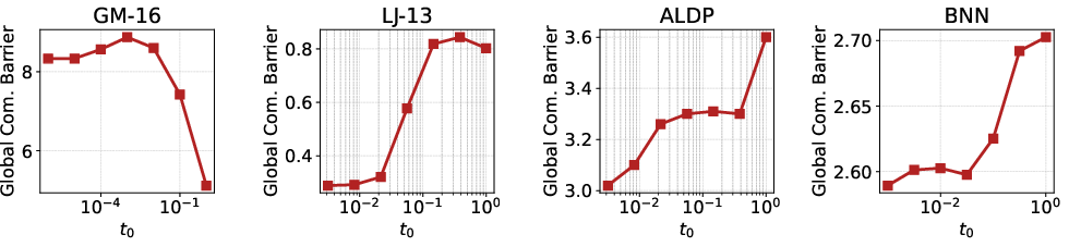
- It improves how well Parallel Tempering communicates between the easy and hard distributions by choosing a small—but not too small—starting time t0. Small t0 helps, because the in‑between distribution is closer to the easy reference and easier to explore. But if t0 is too tiny, things become too concentrated, which can hurt efficiency.
- Using the SDE to transport samples (Stage 2) consistently beats a simpler shortcut (directly “inverting” the map). The SDE actively corrects and improves samples as they move, while the shortcut can magnify small mistakes.
They tested CDS on eight targets across four types of tasks:
- Gaussian mixtures (2D and 16D; classic multi‑peak tests),
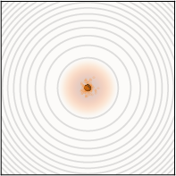
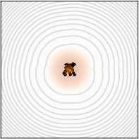
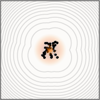
- Lennard‑Jones particle clusters (physics; 39 and 165 dimensions),
- Alanine dipeptide (a small molecule in 66 dimensions; common in molecular simulation),
- A Bayesian neural network posterior (550 dimensions; large and tricky).
Across these, CDS often matched or outperformed state-of-the-art methods, especially when the budget of density evaluations was tight (which is common in real applications).
Why it matters:
- Many scientific and machine learning problems rely on drawing diverse, accurate samples from tough distributions—like exploring molecule shapes or estimating uncertainty in neural networks.
- Every density evaluation can be expensive (e.g., simulating forces between atoms or running a big model). CDS gives you more “bang for your buck.”
What this could change (implications)
- Faster scientific simulations: In chemistry, physics, and biology, CDS could reduce compute time while still exploring all important configurations (peaks).
- Better uncertainty estimates: In Bayesian machine learning, CDS can sample from complex posteriors without costly training phases.
- Practical and plug‑and‑play: Because there’s no neural training and the key math pieces have closed‑form expressions, CDS can be easier to adopt and tune.
- Future improvements: The idea of “conditional paths” could be paired with different paths, schedules, or samplers. Picking t0 well and designing even better paths may improve performance further.
In short, the paper shows a clever way to combine a reliable explorer (Parallel Tempering) with an exact, learning‑free transporter (diffusion SDE) to sample efficiently from hard, multi‑peak distributions. It’s precise, practical, and often more cost‑effective than current methods.
Knowledge Gaps
Knowledge gaps, limitations, and open questions
The paper proposes Conditional Diffusion Sampling (CDS) and demonstrates promising empirical performance, but several aspects remain unaddressed or only partially explored. The following list summarizes concrete gaps and open questions that future work could tackle:
- Exactness and bias control:
- What conditions (on Stage 1 and Stage 2) guarantee asymptotically exact sampling from the target as computation increases?
- How large is the residual bias from finite PT steps, SDE discretization, and finite corrector steps, and how does it scale with dimension and target curvature?
- Can a global Metropolis–Hastings correction (e.g., pathwise or at final time) render CDS unbiased?
- Initialization time selection:
- How to choose or adapt the initial time in a principled way (e.g., based on overlap, round trips, or estimated communication barriers)?
- Can one derive theoretical or data-driven criteria for the optimal as a function of target geometry and dimensionality?
- Noise and time schedules:
- How should the diffusion noise schedule and the time grid be optimized or adapted online for stability, accuracy, and cost?
- Are there provably optimal or near-optimal schedules for given classes of targets?
- Interpolant design beyond linear:
- How to construct task- or geometry-aware conditional interpolants that avoid the pathologies observed with linear paths (e.g., particle collisions in molecular systems)?
- Can one design manifold-aware or symmetry-preserving interpolants (e.g., for toroidal angles, permutation symmetries of LJ clusters)?
- What criteria (e.g., Lipschitz constants, condition numbers, or transport cost) best predict the efficiency of a given ?
- Stability near singularities:
- The score and velocity fields blow up as ; what step-size controls, time-warpings, or regularizations ensure stable integration?
- How to rigorously bound numerical error and stability for stiff potentials and heavy-tailed targets?
- Discretization and solver choices:
- What is the impact of higher-order SDE integrators or adaptive time-stepping on efficiency and accuracy?
- Can implicit or variance-reduced schemes improve stability near small without excessive cost?
- Corrector design:
- Which MCMC correctors (e.g., MALA, HMC, Riemannian variants, or preconditioned proposals) yield the best trade-off along the conditional path?
- How many corrector steps are needed at each , and can this be chosen adaptively based on local error or acceptance rates?
- Stage 1 sampler and schedule:
- While PT is used, are there cases where SMC/AIS or hybrid strategies outperform PT for sampling ?
- How to automatically tune tempering schedules specifically for the conditional target family ?
- Reference distribution sensitivity:
- How sensitive is CDS to the choice of reference distribution fails to cover regions that map to important modes, can CDS still recover them?
- Can learned or adapted references (e.g., flows, variational approximations) improve coverage and reduce sensitivity?
- Dependence on anchor choices:
- How does mode coverage depend on the sampled anchor ? Are multiple anchors per run or anchor diversification strategies beneficial?
- Can one design anchor selection policies that target under-explored regions or leverage prior structure?
- Gradient requirements and cost accounting:
- CDS relies on exact gradients of ; how does it perform with noisy or approximate gradients (e.g., stochastic mini-batches in BNNs)?
- What is a fair computational budget metric that accounts for both density and gradient evaluations across methods?
- Theoretical guarantees:
- Formal conditions for existence/uniqueness of solutions to the conditional SDE and regularity of the induced path densities.
- Mixing-time or convergence-rate analyses for CDS versus PT or other samplers, especially in high dimensions.
- Robustness and generality:
- Behavior on heavy-tailed, bounded-support, or non-smooth targets where scores may be ill-behaved.
- Extension to constrained or manifold-valued domains (e.g., torus, simplex, SPD manifolds) with appropriate diffeomorphic and SDEs.
- Discrete or mixed-variable targets:
- Can CDS be extended to discrete spaces or mixed continuous–discrete models (e.g., via relaxations or piecewise-defined interpolants)?
- Evidence (normalizing constant) estimation:
- Can the conditional path be exploited for estimating (e.g., via path sampling or Jarzynski-like identities), and what are the variance properties?
- Budget allocation:
- How to optimally allocate computation between Stage 1 (global exploration) and Stage 2 (transport/correction) for different targets and budgets?
- Can adaptive controllers re-allocate effort online based on diagnostics?
- Diagnostics and monitoring:
- Beyond PT round trips, what diagnostics are informative for CDS (e.g., overlap metrics along the path, ESS for correctors, pathwise divergences)?
- Can these be used to adapt schedules, , or corrector steps on the fly?
- SDE vs ODE transport:
- When does deterministic transport (σ_t=0) outperform stochastic transport, and can hybrid or stage-dependent choices be beneficial?
- What are the trade-offs in multi-modal settings where stochasticity may aid barrier crossing?
- Symmetry and invariance:
- How to ensure and the dynamics respect model symmetries (e.g., particle permutations, translational/rotational invariance) to improve efficiency?
- Scaling laws and high-dimensional behavior:
- Empirical and theoretical scaling with dimension (beyond D=550), curvature, and multimodality complexity.
- Memory/compute trade-offs for large-batch parallelization over anchors and trajectories.
- Fair and comprehensive comparisons:
- A principled analysis of why CDS scales better than other non-amortized diffusion-based samplers (e.g., RDMC, DiGS) in high dimensions, including matched cost models.
- Semi-amortized extensions:
- Although CDS is training-free, can lightweight learned interpolants or schedule predictors be trained with modest budgets to further reduce correction costs?
- Multi-target or sequential settings:
- Reusing anchors, references, or interpolants across related targets (e.g., tempering chains of models) to amortize exploration.
- Hard constraints and projections:
- Incorporating bond-length or other hard constraints (common in molecular systems) via constrained SDEs or projection steps within CDS.
These gaps suggest avenues for theory, algorithms, and applications to make CDS more principled, robust, and broadly applicable.
Practical Applications
Immediate Applications
The following applications can be deployed now using the paper’s algorithmic contributions (Conditional Diffusion Sampling, CDS) and the released code. Each item names the use case, explains how CDS would be used, links sectors, notes expected benefits, and lists key assumptions/dependencies.
- Faster posterior sampling for Bayesian Neural Networks (BNNs) with limited compute
- Sectors: software/ML, healthcare (diagnostic uncertainty), finance (risk models), robotics (safety-aware control)
- How to use: Replace HMC/MALA or plain PT with CDS for BNN posterior sampling; use the linear conditional interpolant, run Stage 1 (PT on ν_{t0|z}) + Stage 2 (closed-form SDE integration) to get calibrated uncertainty with fewer log-density/gradient evaluations.
- Tools/workflows: PyTorch/JAX BNNs with autodiff for ∇log π; integrate as a custom sampler in PyMC, NumPyro, TFP, or BlackJAX.
- Benefits: Better sample quality per density evaluation vs. state-of-the-art MCMC; robust on high-dimensional, multimodal posteriors (demonstrated at D=550).
- Assumptions/dependencies: Requires access to log-posterior and gradients; target is continuous on ℝD; modest tuning of t0 and PT schedule.
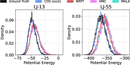
- Accelerated sampling of molecular conformations and energy landscapes (e.g., Alanine dipeptide, Lennard‑Jones clusters)
- Sectors: healthcare/drug discovery, materials, chemistry
- How to use: Wrap force-field energy/gradient calls (e.g., OpenMM, ASE) as π, run CDS to explore conformational basins and capture multimodal Ramachandran plots within limited force evaluations; use a safe t0 (not too small) to avoid atom overlap under linear interpolation.
- Tools/workflows: OpenMM/ASE + CDS sampler; workflow to select t0 via round-trip diagnostics; periodic MCMC corrector steps for numerical stability.
- Benefits: Captures multiple modes under tight evaluation budgets; competitive with Non-Reversible PT while reducing evaluations.
- Assumptions/dependencies: Differentiable energy function; linear interpolant can be used but may need conservative t0 for short-range repulsions (Lennard‑Jones).
- Improved uncertainty quantification for expensive physics-based models (e.g., climate, astrophysics, engineering calibration)
- Sectors: energy, climate science, aerospace, manufacturing
- How to use: Use CDS to sample multimodal posteriors when each likelihood/prior evaluation is expensive (e.g., PDE solves); Stage 1 improves global exploration via easier conditional bridging, Stage 2 transports without learned surrogates.
- Tools/workflows: Existing simulator wrapped in JAX/PyTorch for gradients or adjoints; schedule optimized by round-trip counts.
- Benefits: Reduces the number of simulator calls for a target accuracy; less sensitive to poor reference–target overlap than plain PT.
- Assumptions/dependencies: Access to gradients (adjoints, autodiff, or differentiable surrogates); continuous targets; careful t0 selection.
- New sampler backend in probabilistic programming systems for multimodal targets
- Sectors: software/ML, academia
- How to use: Add CDS as a backend kernel in PyMC/NumPyro/TFP/BlackJAX for models where NUTS/HMC stalls across modes; expose t0, noise schedule, and corrector steps; auto-tune via round-trip statistics.
- Tools/products: “CDS-PTSampler” module with API parity to existing kernels; heuristics to pick t0 maximizing round trips subject to non-degeneracy.
- Benefits: Turnkey gains on multimodal models without training neural samplers; integrates with existing diagnostics (ESS, R-hat, RTs).
- Assumptions/dependencies: Models yield ∇log π; supports only continuous variables out of the box.
- Econometrics and epidemiology: robust inference in mixture/regime-switching models
- Sectors: finance, public health, policy analysis
- How to use: Apply CDS to mixture posteriors (e.g., stochastic volatility with regimes, epidemic models with multi-peak likelihoods) to avoid mode trapping.
- Tools/workflows: Implement in PPL of choice; use linear interpolant; track round trips as a mixing KPI.
- Benefits: Better coverage of posterior modes under fixed computational budgets, improving risk estimates and scenario analyses.
- Assumptions/dependencies: Differentiable likelihoods or reparameterizations for gradients.
- Risk and pricing engines in quantitative finance (e.g., VaR under multimodal priors)
- Sectors: finance
- How to use: CDS to draw samples for tail risk estimation when models induce multi-modality (jumps, regime-switching); integrate with nightly batch pipelines to reduce compute.
- Tools/workflows: JAX/PyTorch modeling stack; GPU-accelerated CDS; budget-aware scheduling (allocation between Stage 1 and Stage 2).
- Benefits: Lower cost for a given error in tail metrics; improved robustness across market regimes.
- Assumptions/dependencies: Differentiable model components or adjointable SDE solvers.
- Teaching and benchmarking toolkit for multimodal sampling
- Sectors: academia/education
- How to use: Use CDS code and the paper’s tasks (GM, LJ, ALDP, BNN) to teach annealing, tempering, diffusion transport, and round-trip diagnostics.
- Tools/products: Ready-to-run notebooks comparing CDS vs. PT/HMC/MALA; plug-in metrics (Wasserstein-2, KL of Ramachandran, energy histograms).
- Benefits: A reproducible suite demonstrating practical trade-offs among samplers.
- Assumptions/dependencies: None beyond the released code and standard ML/science Python stack.
Long-Term Applications
These applications will likely require further research or engineering (e.g., new interpolants, constraints handling, or scaling).
- Constraint-aware CDS for large biomolecules and materials (bond/angle constraints, manifolds)
- Sectors: drug discovery, structural biology, materials
- Vision: Design conditional interpolants that preserve bond lengths/angles or operate on torsion manifolds; avoid unphysical overlaps as t → 0; integrate with enhanced sampling (e.g., collective variables).
- Tools/products: “CDS-ConfGen” plugin for OpenMM with constraint-preserving interpolants; adaptive t0 set by overlap metrics; domain priors in reference distribution.
- Dependencies: Derivation of manifold-aware conditional interpolants and scores; robust Jacobian computations; validation on proteins and solids.
- CDS-assisted training of neural samplers (amortized inference at low cost)
- Sectors: software/ML, healthcare, finance
- Vision: Use CDS to generate high-quality, low-budget samples to train diffusion/flow-based neural samplers; amortize over repeated inference tasks while cutting training density evaluations.
- Tools/products: “CDS→NeuralSampler” pipeline; active selection of t0 and schedules to maximize sample diversity for training.
- Dependencies: Curriculum over targets; stability of teacher-student training; metrics for optimal data generation.
- Extensions to mixed/discrete or combinatorial posteriors
- Sectors: operations research, genomics, network science
- Vision: Generalize conditional interpolants to mixed discrete–continuous spaces (e.g., via relaxations or auxiliary variables) to handle graph structures, sequence models, or combinatorial designs.
- Tools/products: Gumbel-relaxed or piecewise-constant conditional paths; hybrid PT on auxiliary variables + SDE on continuous parts.
- Dependencies: Theoretical guarantees for non-Euclidean/relaxed spaces; efficient Jacobian/score surrogates.
- Adaptive, self-tuning CDS (Auto-CDS)
- Sectors: software/ML tooling, academia
- Vision: Online optimization of t0, temperature ladder, noise schedule, and K/N budget split using round-trip counts, acceptance statistics, and error proxies; automatic failure detection for degeneracy (t0 too small).
- Tools/products: Auto-tuner integrated into PPLs; dashboards tracking global communication barriers and Pareto progress.
- Dependencies: Reliable, low-variance diagnostics; multi-objective controllers; cross-model generalization.
- Multi-fidelity and surrogate-assisted CDS for simulator-based inference
- Sectors: climate, aerospace, energy
- Vision: Couple CDS with learned surrogates or reduced-order models in Stage 1, then correct with high-fidelity gradients in Stage 2; use control variates to cut variance/evaluations.
- Tools/products: Surrogate manager for density/gradient calls; error-aware switching between fidelities.
- Dependencies: Trust-region or error-bounded surrogates; guarantees on bias correction.
- Real-time uncertainty quantification in autonomous systems
- Sectors: robotics, autonomous driving, industrial automation
- Vision: Use CDS to maintain calibrated posteriors under tight latency budgets (e.g., safety-critical decision loops) by spending most compute on quick Stage 1 exploration then short SDE refinements.
- Tools/products: GPU-optimized kernels for CDS; anytime variants that return progressively refined samples.
- Dependencies: Low-latency gradient computation; bounded-time solvers; safety certification.
- Hardware and systems integration
- Sectors: HPC, cloud, edge
- Vision: Highly optimized GPU/TPU kernels for conditional score evaluation (via change of variables) and SDE integration; elastic scaling of Stage 1 PT replicas on clusters.
- Tools/products: CUDA/JAX/TFP implementations; Kubernetes operators that adapt K/N based on budget.
- Dependencies: Efficient Jacobian/score codegen; numerical stability across large replica counts.
- Policy and governance: standardized UQ with bounded budgets
- Sectors: public policy, regulatory science
- Vision: Incorporate CDS into methodological toolkits for policy models (epidemiology, macroeconomics) where compute is constrained; report round-trip-based diagnostics as transparency measures.
- Tools/products: Open templates for policy analyses with budgeted sampling plans; audit trails linking budget to posterior accuracy.
- Dependencies: Gradient access for policy models (or differentiable surrogates); training analysts on CDS diagnostics.
Cross-cutting assumptions and dependencies affecting feasibility
- Gradient access: CDS requires ∇log π of the target; if the model is not differentiable, one needs adjoints, reparameterizations, or differentiable surrogates. Finite differences are possible but may negate CDS’s efficiency gains.
- Domain and support: Current derivations target continuous variables on ℝD. Constrained or manifold supports require specialized conditional interpolants; discrete variables need relaxations or auxiliary-variable schemes.
- Initialization choice t0: Must be small enough to boost overlap and round trips, but not so small that the conditional path degenerates. Practical workflow: tune t0 by monitoring round trips and sampling error.
- Interpolant choice: Linear interpolant is simple and effective, but can be unsafe for strong short-range interactions (e.g., Lennard‑Jones). Domain-informed interpolants reduce path pathologies.
- Budgets and splits: Performance depends on allocating compute between Stage 1 (PT steps K) and Stage 2 (SDE steps N and corrector steps M). Auto-tuning helps in production settings.
- Numerical stability: Euler–Maruyama works but may require corrector steps; stiff targets may benefit from better SDE solvers or adaptive step sizes.
Glossary
- Annealed Importance Sampling (AIS): A method that transports weighted particles through an annealing sequence from a reference to a target distribution. "Annealed Importance Sampling (AIS, \cite{neal2001annealed})"
- Annealing-based methods: Techniques that introduce a sequence of intermediate distributions bridging a reference and target to improve mixing. "Annealing-based methods differ in how they navigate this sequence."
- Change of variables formula: A rule for transforming probability densities under invertible mappings using the Jacobian determinant. "change of variables formula:"
- Conditional Diffusion: A diffusion process defined on a conditional probability path whose SDE preserves the path’s marginals. "we define the corresponding Conditional Diffusion via the following SDE:"
- Conditional Diffusion Sampling (CDS): The proposed two-stage framework combining PT-based initialization with closed-form conditional diffusion transport. "Conditional Diffusion Sampling (CDS), a framework that combines these two paradigms."
- Conditional Interpolants: Interpolant processes defined conditionally on a reference sample that induce a tractable conditional path of distributions. "Conditional Interpolants, a class of stochastic processes"
- Continuity equation: A PDE describing conservation of probability mass under deterministic flows. "with marginals satisfying the continuity equation."
- Diffeomorphism: A smooth, bijective map with a smooth inverse, ensuring well-defined change-of-variables. "the map is a diffeomorphism."
- Diffusive Gibbs Sampling (DiGS): A non-amortized sampler introducing Gaussian convolutions to encourage cross-mode moves. "Diffusive Gibbs Sampling (DiGS, \cite{chen2024diffusive}) introduces Gaussian convolutions"
- Dirac delta: A distribution concentrated at a single point, representing a point mass. "a Dirac delta centered at "
- Displacement interpolant: The geodesic interpolation of measures in optimal transport between two distributions. "corresponds to the displacement interpolant between and "
- Drift vector field: The deterministic component of an SDE governing the direction of motion. "is the drift vector field"
- Euler--Maruyama scheme: A numerical method for discretizing and simulating SDEs. "We use the Euler--Maruyama scheme to integrate the SDE"
- Fokker-Planck-Kolmogorov (FPK) equation: A PDE that governs the time evolution of the probability density of a diffusion. "the Fokker-Planck-Kolmogorov (FPK) equation"
- Flow matching frameworks: Approaches that learn vector fields to match probability flows between distributions. "This is the canonical choice in flow matching frameworks"
- Geometric path: An annealing path where intermediate densities are geometric averages of reference and target densities. "A common choice is the geometric path"
- Hamiltonian Monte Carlo (HMC): An MCMC algorithm using Hamiltonian dynamics to propose distant, high-acceptance moves. "Hamiltonian Monte Carlo (HMC, \citet{duane1987hybrid})"
- Hypervolume Ratio (HVR): A normalized measure of Pareto front quality in multi-objective evaluation. "Mean Hypervolume Ratio (HVR)"
- Itô diffusion process: A stochastic process solution to an SDE in the Itô calculus framework. "is an (Itô) diffusion process"
- Jacobian matrix: The matrix of first-order partial derivatives of a vector-valued function, used in density transformations. "the Jacobian matrix of the map "
- Kullback–Leibler (KL) divergence: A measure of discrepancy between probability distributions. "the Kullback-Leibler (KL) divergence between Ramachandran plots"
- Lennard–Jones (LJ): A potential model for interactions between particles in physical systems. "Comparison of Lennard-Jones (LJ) potential energy histograms."
- Lipschitz constant: A bound on how much a function can stretch distances, relevant to contraction/expansion effects. "let be the Lipschitz constant of the interpolant ."
- Markov Chain Monte Carlo (MCMC): A family of algorithms constructing Markov chains with a desired invariant distribution. "Markov Chain Monte Carlo (MCMC, \cite{meyn2012markov}) methods aim to sample"
- Markov kernel: A stochastic transition rule defining probabilities of moving between states. "Let be any Markov kernel invariant with respect to ."
- Metropolis–Adjusted Langevin Algorithm (MALA): An MCMC method combining Langevin dynamics with Metropolis correction for proposals. "Metropolis--Adjusted Langevin Algorithm (MALA)"
- Metropolis–Hastings (MH): A general MCMC algorithm that accepts or rejects proposals to ensure target invariance. "Metropolis--Hastings (MH, \citet{metropolis1953equation,hastings1970monte})"
- Metropolis-within-Gibbs: A hybrid scheme embedding Metropolis updates within a Gibbs sampling structure. "Metropolis-within-Gibbs procedure"
- Neural Diffusion Samplers: Diffusion-inspired samplers that learn transport using the target density and samples. "via Neural Diffusion Samplers \cite{akhound2024iterated,nusken2024transport,albergo2025nets,akhound2025progressive,zhang2025accelerated}."
- Non-Reversible PT (NRPT): A variant of Parallel Tempering that uses non-reversible dynamics to improve mixing. "Non-Reversible PT (NRPT)"
- Noise schedule: A time-dependent specification of diffusion strength in stochastic processes. "The noise schedule controls the path stochasticity"
- Ordinary Differential Equation (ODE): A deterministic differential equation governing flow-based transport when diffusion vanishes. "Ordinary Differential Equation (ODE)"
- Parallel Tempering (PT): An annealing-based MCMC method running multiple replicas at different temperatures with swap moves. "Parallel Tempering (PT) serves as the gold standard"
- Pareto fronts: The set of solutions representing optimal trade-offs in multi-objective evaluation. "Pareto fronts for sampling performance"
- Pushforward: The distribution obtained by transforming a random variable through a function. "as the pushforward of through ."
- Ramachandran plots: Angular distributions used to assess protein conformations (e.g., phi/psi angles). "the Kullback-Leibler (KL) divergence between Ramachandran plots for ALDP"
- Reverse Diffusion Monte Carlo (RDMC): A method leveraging reverse-time diffusion and score expectations, approximated via nested MCMC. "Reverse Diffusion Monte Carlo (RDMC, \cite{huang2024reverse}) expresses the score"
- Round Trips (RTs): A measure of PT communication efficiency counting full traversals between reference and target replicas. "Round Trips (RTs)"
- Score function: The gradient of the log-density guiding score-based dynamics or corrections. "the score function, , does not need to be learned."
- Sequential Monte Carlo (SMC): A particle-based method propagating and resampling weighted populations along an annealing path. "Sequential Monte Carlo (SMC, \cite{del2006sequential})"
- Stochastic differential equation (SDE): A differential equation with randomness (e.g., driven by a Wiener process) defining diffusions. "stochastic differential equation (SDE)"
- Stochastic Interpolants: A framework that defines processes by interpolating between samples, unifying flows and diffusions. "Stochastic Interpolants"
- Velocity field: The vector field giving the instantaneous rate of change of states along an interpolant or flow. "the conditional velocity field "
- Wasserstein-1 distance: An optimal transport metric measuring the cost to move mass between distributions. "Wasserstein-1 distance"
- Wasserstein-2 () distance: The quadratic-cost version of the Wasserstein distance used to assess sample quality. "the Wasserstein-2 () distance"
- Wiener process: A continuous-time Gaussian process (Brownian motion) driving the noise in SDEs. " is a -dimensional Wiener process."
Collections
Sign up for free to add this paper to one or more collections.