Frequency Shift Physics-Informed Extreme Learning Machine for Solving High-Frequency Partial Differential Equations
Abstract: Solving partial differential equations (PDEs) with high-frequency solutions remains a central challenge in physics-informed machine learning due to spectral bias -- the tendency of neural networks to learn low-frequency components preferentially. This paper proposes a Frequency Shift Physics-Informed Extreme Learning Machine (FS-PIELM) framework that addresses this limitation through an additive mechanism for weight initialization. Rather than multiplying random weights by a scaling factor, the method translates the mean of the Gaussian weight distribution while keeping the variance fixed at unity, thereby avoiding the variance amplification inherent in scaling-based methods. Two variants are developed: FS-PIELM-L assigns independent frequency magnitudes to individual neurons, while FS-PIELM-G groups neurons for improved robustness. Theoretical analysis shows that the frequency variance under the proposed framework remains bounded and approaches unity regardless of target frequency, in contrast to the quadratic growth of conventional approaches. The method preserves the computational efficiency of extreme learning machines, requiring only a single linear solve. Experiments on seven benchmark problems spanning six equation types -- Helmholtz, wave, Poisson, Klein-Gordon, heat, and advection-diffusion -- on both regular and complex geometries show that the linear variant achieves the best accuracy in six of seven cases, with improvements of one to nearly five orders of magnitude over existing PIELM variants. The code and data accompanying this manuscript will be made publicly available at https://github.com/xgxgnpu/Physics-informed-vibe-coding/tree/main/FS-PIELM.
Paper Prompts
Sign up for free to create and run prompts on this paper using GPT-5.
Top Community Prompts
Explain it Like I'm 14
What is this paper about?
This paper introduces a faster and more accurate way to solve math problems called partial differential equations (PDEs), especially when their answers wiggle or oscillate a lot (think of sound waves or ripples on water). The new method is called Frequency Shift Physics-Informed Extreme Learning Machine (FS-PIELM). It teaches a simple type of neural network to follow the rules of physics while avoiding a common problem where networks prefer to learn smooth, slow-changing patterns and struggle with fast, high-frequency details.
What questions does the paper try to answer?
- How can we make neural networks solve “wiggly” (high-frequency) physics problems more accurately?
- Can we do this without making training slow or complicated?
- Is there a smarter way to give the network the right “frequencies” so it learns sharp details without getting confused or unstable?
How did the researchers do it?
First, a simple idea: many PDEs describe real-world physics (like heat, sound, or waves). To solve them with machine learning, you can train a network to produce answers that follow the equation and the boundary rules (what happens on the edges of the region). That’s called physics-informed learning.
The paper uses a very fast kind of network called an Extreme Learning Machine (ELM):
- It has one hidden layer.
- The hidden-layer weights are chosen randomly and then kept fixed.
- Only the final layer is learned, and it’s solved in one shot using linear algebra (no long training loops). This makes it very fast.
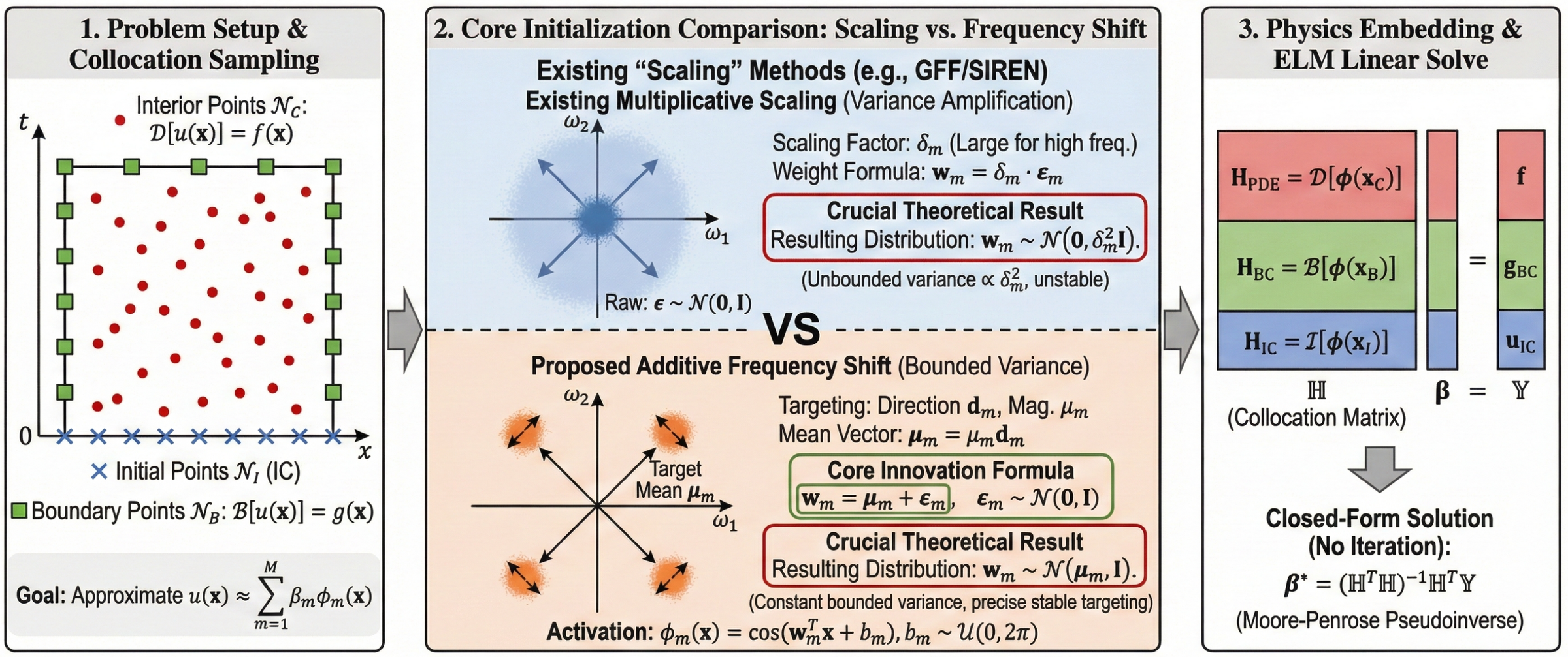
The challenge: neural networks tend to learn low-frequency (smooth) parts first and struggle with high-frequency details. Older fixes often “multiply” the inputs to force higher frequencies. But multiplying also makes the randomness blow up a lot—like turning up the volume so high that you add lots of noise. That makes high-frequency learning unstable.
The new trick in FS-PIELM is different:
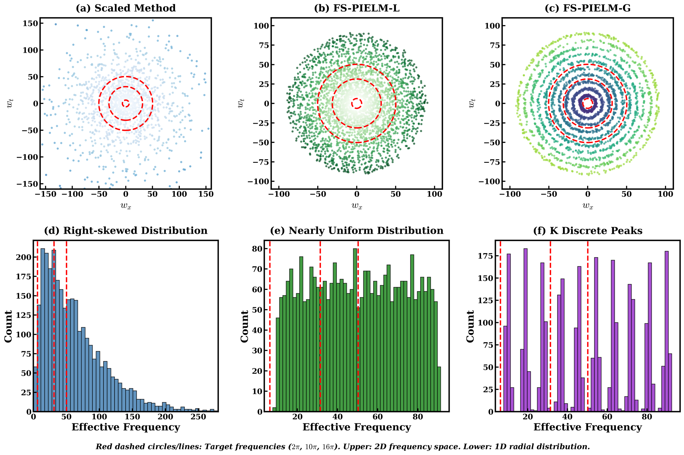
- Instead of multiplying, it “shifts” the center (the mean) of the random weights to aim each neuron at a certain frequency, while keeping the spread (the variance) steady and well-behaved.
- Think of tuning a radio: older methods turned the volume knob to try to get a station; FS-PIELM turns the tuning knob to the right station directly, without cranking the volume.
- Each neuron gets:
- A random direction (so all spatial directions are covered fairly).
- A target frequency size (its “station”).
- A small, controlled amount of randomness.
- Two versions:
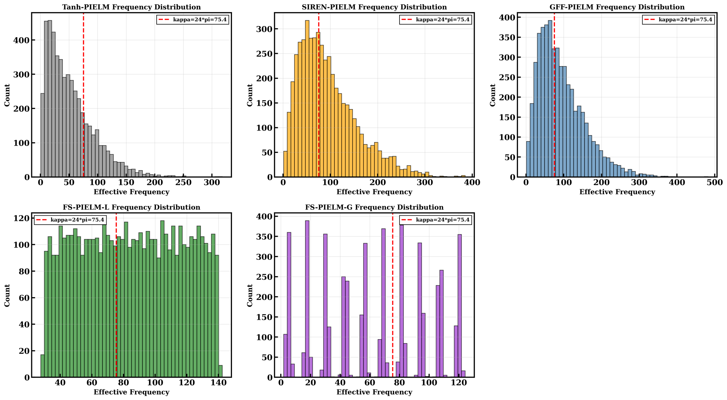
- FS-PIELM-L (Linear): gives each neuron its own frequency, filling the whole range finely.
- FS-PIELM-G (Grouped): groups neurons so several share the same frequency, which can be more robust but a bit less precise.
Why this helps (in simple terms):
- Multiplying to reach higher frequencies also multiplies how much the random parts jump around—this variance grows a lot, making things unstable at high frequencies.
- Shifting the mean to target a frequency keeps the randomness under control (its variance stays about the same), even at very high frequencies.
- Mathematically, the “spread” of the actual frequencies the neurons produce stays bounded (roughly constant), instead of growing with the target frequency.
What did they find?
The team tested their method on seven tough problems, including:
- Helmholtz and wave equations (common in acoustics and vibrations),
- Poisson and Klein–Gordon equations,
- Heat and advection–diffusion equations,
- Both simple and complex shapes.
Here’s what stood out:
- FS-PIELM-L (the linear version) was the most accurate in 6 out of 7 tests.
- It beat strong alternatives (like SIREN-PIELM and GFF-PIELM) by about 10 times to almost 100,000 times in error reduction, depending on the problem.
- It stayed fast: you still solve everything with one linear system, so results arrive in seconds on a CPU.
- It was less sensitive to parameter choices (more robust), meaning it worked well across a wider range of settings.
- The grouped version (FS-PIELM-G) was slightly less accurate but often more stable.
Why this matters:
- For high-frequency problems (lots of wiggles), older methods waste many neurons on the wrong frequencies or spread them too widely.
- FS-PIELM packs neurons tightly around the frequencies that matter, like assigning instruments in an orchestra to the exact notes in the score rather than random notes around them.
Why is this important?
This approach makes solving complex physics problems:
- More accurate for high-frequency details (like sharp wave patterns),
- Faster and simpler to train (no long gradient descent),
- Easier to tune (fewer fragile settings),
- Useful across many areas: acoustics, electromagnetics, structural vibrations, heat transfer, and fluid flow.
If you care about engineering simulations, scientific computing, or learning model parameters from limited data, this method can give you better answers with less hassle. The authors also plan to share their code, making it easier for others to use and build upon.
Key ideas in plain language
- Partial Differential Equation (PDE): A math rule that tells how something changes in space and/or time (like how heat spreads or how waves move).
- Frequency: How quickly something oscillates; higher frequency = more wiggles in the same space.
- Spectral bias: Neural networks naturally prefer smooth, slow-changing patterns and struggle with fast oscillations.
- Extreme Learning Machine (ELM): A fast network that picks hidden-layer weights randomly and solves the final layer in one shot.
- Frequency shift (this paper’s idea): Aim neurons directly at the right frequencies by shifting the center of their weights, instead of multiplying inputs (which adds too much randomness).
A simple analogy
Imagine trying to listen to a specific radio station:
- Old methods: turn up the volume to try to “hear” the station—this also boosts static (noise).
- FS-PIELM: turn the tuning knob to the exact station and keep the volume at a reasonable, steady level. You hear the station clearly without extra noise.
That’s what this paper does for high-frequency physics problems: it tunes the network to the right frequencies cleanly and efficiently.
Knowledge Gaps
Knowledge gaps, limitations, and open questions
The following list captures what remains missing, uncertain, or unexplored in the paper and can inform concrete future research directions:
Theory and guarantees
- Lack of approximation and convergence guarantees: No bounds relate solution error (e.g., PDE residual or error) to the number of neurons , collocation density, and frequency parameters for FS-PIELM.
- Conditioning and identifiability: No analysis of the conditioning of the collocation matrix as increases, nor of how truncated SVD thresholds or Tikhonov regularization affect stability and accuracy at high frequencies.
- Kernel viewpoint and expressivity: The paper does not characterize the implicit kernel induced by mean-shifted cosine random features (via Bochner’s theorem) or connect spectral choices to target PDE spectral measures for guaranteed representation.
- Variance analysis precision: The frequency-variance result uses a delta-method approximation; exact expressions (and dimension-dependent concentration results) for are not derived, nor is the coefficient of variation formalized to quantify concentration at high .
- Nonlinear PDEs: Theoretical guarantees and training formulations for nonlinear operators (where the ELM linear-solve advantage no longer holds) are not provided.
Method design and hyperparameters
- Automated frequency selection: The method relies on linear spacing of within chosen by grid search. No automatic or data-/residual-driven procedure exists to select or adapt online (e.g., wavenumber estimation, residual-spectrum matching, band allocation).
- Band allocation strategy: Only linear spacing is considered; alternative allocations (e.g., logarithmic, clustered around estimated dominant wavenumbers, or problem-adaptive spacing across groups K) are unexplored.
- Anisotropic frequency control: Inputs are treated isotropically. For problems with distinct spatial/temporal scales, anisotropic frequency control (per-dimension or anisotropic covariance) is not studied.
- Choice of activation and bias distribution: Cosine with is fixed. The effect of bias distributions, mixed sine/cosine features, or learnable phases on accuracy and conditioning is unexamined.
- Variance of the Gaussian perturbation: The variance is fixed at unity. The impact of tuning perturbation variance (or using non-identity covariances) on approximation, robustness, and conditioning is not assessed.
- Grouping strategy hyperparameters: The number of groups , group sizes, and adaptive grouping policies are not studied systematically beyond a single choice (e.g., ).
Numerical stability, sampling, and scalability
- Collocation density vs. resolvable frequency: There is no guideline connecting collocation point density and distribution to the highest targeted frequency (Nyquist-like criteria for PDE residuals), nor study of aliasing and under-sampling effects.
- Preconditioning and normalization: Large factors enter derivative operators (e.g., Laplacian). Strategies to normalize basis derivatives, scale PDE rows, or precondition to mitigate dynamic-range issues are not provided.
- Large-scale solvers: For very large and , memory/time constraints of SVD are not addressed. Alternatives (randomized SVD, iterative least-squares with preconditioning, sketching) are not explored.
- Sensitivity to SVD cutoff: A fixed threshold () is used. Its effect on accuracy, stability, and reproducibility across problems and frequency ranges is not studied.
Scope and benchmarks
- High-dimensional settings: Performance, sampling, and directional concentration effects for are not evaluated; the number of neurons and collocation points needed as a function of dimension remains unclear.
- Irregular geometries and boundary types: While claimed, detailed tests on complex geometries and diverse boundary conditions (Neumann, Robin, mixed, interface conditions) are not presented in the provided content.
- Variable-coefficient and anisotropic PDEs: The effect of medium heterogeneity and anisotropy on directional sampling (uniform on the sphere) and on the optimal frequency distribution is not studied.
- Non-smooth features: Behavior on discontinuities, shocks, or sharp layers (e.g., advection-dominated problems) is not examined; cosine features may struggle without domain decomposition or local adaptivity.
- Comparative breadth: Comparisons are limited to PIELM variants. Performance relative to strong PINN baselines (e.g., deep SIREN PINNs, adaptive Fourier features) and classical solvers (e.g., -FEM, spectral elements) is absent.
Extensions and use cases
- Nonlinear and coupled systems: Experiments and formulations for nonlinear PDEs (e.g., nonlinear Klein–Gordon, Navier–Stokes) or coupled systems are not provided; how FS-PIELM integrates with iterative solvers for nonlinear residuals remains open.
- Inverse problems and noisy data: The method is not evaluated on inverse problems, parameter inference, or data assimilation with noisy/limited observations.
- Adaptive sampling: No residual-based collocation refinement or active learning is used, despite high-frequency solutions typically benefiting from adaptive point placement near high-residual regions.
- Local/partitioned models: Integration with domain decomposition or localized bases (to better capture spatially varying spectra and complex boundaries) is not explored.
- Time–space separation: For time-dependent PDEs, a unified isotropic sampling in the joint space is implied; optimal strategies for differing temporal and spatial frequency content are not examined.
These gaps suggest concrete follow-ups: develop adaptive frequency and sampling schemes tied to residual spectra; analyze and precondition the collocation system for high- regimes; extend theory to approximation and convergence guarantees; benchmark against strong deep-learning and classical solvers; and test on nonlinear, high-dimensional, anisotropic, and non-smooth PDEs, including inverse settings with noise.
Practical Applications
Immediate Applications
Below are concrete, real-world use cases that can be deployed with the current FS-PIELM framework and codebase, leveraging its single linear-solve training and superior performance on high-frequency PDEs.
- High-frequency acoustics simulation for design and analysis
- Sectors: architecture/engineering (AEC), automotive/aerospace (NVH), consumer audio, underwater acoustics/sonar
- Tools/products/workflows: CPU-based “acoustics quick solver” for room modes, speaker placement, muffler/duct acoustics, underwater sound fields; rapid parametric sweeps in early-stage design; FS-PIELM-L for precise narrowband targeting and FS-PIELM-G when robustness against random initialization is desired
- Assumptions/dependencies: linear Helmholtz model or linearized regime; adequate boundary-condition sampling; 2D/3D feasibility depends on memory and SVD scaling; absorbing boundary conditions may need tailored residual terms
- Photonics and RF preliminary wave analysis (frequency-domain)
- Sectors: electronics, photonics, telecommunications
- Tools/products/workflows: fast surrogate for waveguide/cavity resonance exploration; antenna cavity or photonic crystal preliminary calculations; integrate as a plug-in to Python-based design scripts
- Assumptions/dependencies: scalar-reduced or simplified Helmholtz approximations (not full-vector Maxwell); geometric complexity manageable with mesh-free collocation; boundary/medium heterogeneity explicitly incorporated
- Ultrasound and NDT (non-destructive testing) forward modeling for research and prototyping
- Sectors: healthcare (research), manufacturing QA, materials testing
- Tools/products/workflows: forward simulation of high-frequency wave propagation in homogeneous or mildly heterogeneous media for probe configuration and scenario testing; FS-PIELM-L for fine spectral control
- Assumptions/dependencies: research/prototyping use (not clinical-grade); linear wave models or linearization valid; calibration of μ-range to transducer bandwidth; careful boundary modeling
- Seismic and structural health monitoring (guided-wave) forward solvers
- Sectors: energy (exploration), civil infrastructure, aerospace
- Tools/products/workflows: simulate high-frequency Lamb waves or simplified seismic forward models for crack/damage sensitivity studies and sensor placement; rapid Monte Carlo sweeps for uncertainty studies
- Assumptions/dependencies: simplified 1D/2D forward models; manageable domain sizes; material heterogeneity represented in PDE residual; absorbing/radiation conditions accounted for in collocation
- Environmental noise mapping for urban planning and policy support
- Sectors: public sector, transportation, AEC
- Tools/products/workflows: quick prediction of steady-state noise fields around buildings/infrastructure for scenario comparison; integrate into GIS workflows for what-if analyses
- Assumptions/dependencies: linear acoustics approximation; simplified source/terrain representations; sufficient boundary sampling for irregular geometries
- Fast solvers for advection-diffusion and heat equations in design-of-experiments
- Sectors: chemical/process engineering, HVAC, manufacturing
- Tools/products/workflows: rapid transient or steady predictions for thermal and concentration fields; screening studies and control-oriented prototypes; FS-PIELM-G for robust coverage of ranges of transport Peclet numbers
- Assumptions/dependencies: linear PDEs or linearized operators; controlled domain scaling; stability of SVD with selected collocation density
- Digital twin surrogates for vibro-acoustic subsystems
- Sectors: automotive, aerospace, industrial equipment
- Tools/products/workflows: embed FS-PIELM surrogates inside digital twins to evaluate acoustic/thermal responses at design points; FS-PIELM’s evaluation is fast after training
- Assumptions/dependencies: offline training per operating regime; enough collocation points to capture boundaries and loads; domain decomposition not yet automatic
- Physics-informed inverse modeling with sparse measurements (source recovery, simple parameter inference)
- Sectors: industrial diagnostics, environmental monitoring, R&D
- Tools/products/workflows: augment the residual-based linear system with data misfit rows to infer source terms or scalar parameters; exploit FS-PIELM’s higher fidelity at high frequencies
- Assumptions/dependencies: linear inverse setups or linearized around nominal; measurement noise handling via regularization in SVD; careful conditioning of the collocation matrix
- Education and training: interactive PDE labs
- Sectors: academia, online education
- Tools/products/workflows: classroom demos of high-frequency PDE solutions on CPU laptops; live exploration of wavenumber effects and boundary conditions using the provided open-source code
- Assumptions/dependencies: small to medium problem sizes; basic Python environment and linear algebra libraries; curated examples
- Software integration and productivity tooling
- Sectors: software, CAE/CAD toolchains
- Tools/products/workflows: wrap FS-PIELM inside a Python library/CLI for mesh-free PDE solves; prebuilt templates for Helmholtz, wave, Poisson, advection-diffusion; parameter scans with logging and plotting
- Assumptions/dependencies: reliance on SVD (or truncated SVD) and double precision; moderate memory footprint; user guidance on choosing μmin/μmax (robust but still a hyperparameter pair)
- Uncertainty quantification via repeated solves
- Sectors: R&D, reliability engineering
- Tools/products/workflows: Monte Carlo/UQ loops using FS-PIELM for fast repeated forward solves; prioritized for cases where spectral bias harms alternatives
- Assumptions/dependencies: each sample requires reassembly/solve; consider randomized or incremental SVD for scalability; independence of runs across samples
Long-Term Applications
These opportunities require additional research, scaling, or engineering—e.g., handling large 3D problems, strong nonlinearities, or integrating with complex real-world workflows.
- Large-scale 3D high-frequency acoustics and electromagnetics
- Sectors: aerospace, automotive, telecom, photonics
- Tools/products/workflows: production-grade solvers for cabin acoustics, antenna and cavity design, photonic devices; FS-PIELM as a fast high-frequency basis generator
- Assumptions/dependencies: extension to vector PDEs (Maxwell) and complex media; memory- and time-efficient linear algebra (randomized SVD, iterative solvers); absorbing boundary layers and complex BCs
- Seismic full-waveform inversion (FWI) and tomography at scale
- Sectors: energy, geophysics
- Tools/products/workflows: FS-PIELM as a forward-model surrogate within FWI loops; frequency-band partitioning using FS-PIELM-L to emphasize high-frequency content
- Assumptions/dependencies: strong heterogeneity and nonlinearity; large domains and many sources/receivers; adjoint/sensitivity integration; robust domain decomposition and parallelization
- Real-time digital twins with streaming data assimilation
- Sectors: manufacturing, process control, infrastructure monitoring
- Tools/products/workflows: online updates to FS-PIELM models with sensor data; incremental/online ELM variants for continual learning; closed-loop control
- Assumptions/dependencies: algorithmic development for online updates and noise robustness; stable conditioning of evolving collocation matrices; hardware constraints
- Hybrid FEM/BEM–FS-PIELM workflows (domain decomposition and enrichment)
- Sectors: CAE software, engineering services
- Tools/products/workflows: use FS-PIELM to enrich high-frequency components while FEM/BEM handles low-frequency or complex interfaces; or use FS-PIELM as local solvers in decomposed subdomains
- Assumptions/dependencies: stable coupling strategies, interface conditions enforcement, and error control; automated partitioning and frequency allocation policies
- Automated frequency-band selection and adaptive spectral allocation
- Sectors: software, CAE
- Tools/products/workflows: hyperparameter-free mode where μ-ranges are automatically chosen based on residual spectra; adaptive regrouping (FS-PIELM-G) during training for robustness
- Assumptions/dependencies: residual spectral diagnostics; convergence and stability heuristics; integration with regularization to avoid overfitting
- Advanced inverse problems (heterogeneous properties, distributed sources)
- Sectors: healthcare (imaging R&D), materials, environmental monitoring
- Tools/products/workflows: joint estimation of fields and spatially varying parameters with FS-PIELM priors emphasizing high-frequency fidelity; multi-physics coupling (e.g., thermo-acoustics)
- Assumptions/dependencies: iterative linearization around current estimates; regularization and identifiability; extensions to handle strong nonlinearities
- AR/VR and robotics: real-time acoustic field rendering
- Sectors: consumer tech, gaming, robotics
- Tools/products/workflows: on-device or edge-deployed audio field approximations for spatial audio, echo simulation, or acoustic SLAM; FS-PIELM evaluation is inexpensive once trained
- Assumptions/dependencies: precomputation and compression; fast incremental updates for moving sources/receivers; efficient 3D handling
- Certification-grade clinical and safety applications (ultrasound therapy planning, noise compliance)
- Sectors: healthcare, public policy
- Tools/products/workflows: validated pipelines for therapy planning or regulatory noise assessment; uncertainty bounds and verification/validation artifacts
- Assumptions/dependencies: rigorous V&V against gold-standard solvers; treatment of tissue/medium heterogeneity and attenuation; governance for data and models
- PDE-constrained optimal control with high-frequency physics
- Sectors: energy systems, smart structures, advanced manufacturing
- Tools/products/workflows: embed fast forward models into optimal control loops; explore FS-PIELM-based surrogates with sensitivities
- Assumptions/dependencies: differentiable pipelines and sensitivity analysis; robust handling of constraints and actuator/sensor placement; scalability to high-dimensional control inputs
- Hardware acceleration and embedded deployment
- Sectors: edge computing, IoT
- Tools/products/workflows: specialized linear algebra (GPU/TPU), low-rank solvers, or FPGA-based accelerators for the collocation solve; compressed FS-PIELM models for embedded runtime
- Assumptions/dependencies: integration with vendor BLAS/LAPACK and randomized SVD; memory-aware designs; quantization without harming high-frequency fidelity
- General-purpose PDE solver platforms
- Sectors: scientific computing software, education
- Tools/products/workflows: a user-facing application that auto-detects PDE type, recommends μ ranges, and emits solutions with error estimates; templates for Helmholtz, wave, heat, advection-diffusion on complex geometries
- Assumptions/dependencies: robust geometry handling and BC libraries; adaptive sampling of collocation points; quality metrics guiding users without expert tuning
Glossary
- Advection-diffusion: A partial differential equation modeling combined transport (advection) and spreading (diffusion) of a quantity. Example: "advection-diffusion---on both regular and complex geometries"
- Biharmonic equations: Fourth-order elliptic PDEs involving the Laplacian applied twice, common in plate and elasticity theory. Example: "biharmonic equations \cite{dwivedi2020biharmonic}"
- Boundary condition operator: An operator that enforces boundary constraints on a PDE solution. Example: "\mathcal{B} denotes the boundary condition operator"
- Chi distribution: The distribution of the Euclidean norm of a standard multivariate Gaussian vector. Example: "The chi distribution has \mathbb{E}[|\boldsymbol{\epsilon}|] = c_d"
- Collocation matrix: The matrix formed by evaluating basis functions (and their derivatives) at collocation points for assembling a linear system. Example: "where is the collocation matrix."
- Collocation points: Selected points in the domain and on the boundary where the PDE and boundary conditions are enforced. Example: "at scattered collocation points"
- Delta method: A statistical technique for approximating the variance of a function of a random variable using a Taylor expansion. Example: "Applying the delta method with "
- Dirichlet conditions: Boundary conditions specifying the value of the solution on the boundary. Example: "homogeneous Dirichlet conditions:"
- Domain decomposition: A strategy that splits the computational domain into subdomains to facilitate parallel or localized computation. Example: "domain decomposition \cite{dong2021local,dwivedi2021distributed}"
- Extreme learning machine (ELM): A single-hidden-layer feedforward network with randomly initialized and fixed hidden weights and analytically solved output weights. Example: "The extreme learning machine (ELM) architecture consists of a single hidden layer feedforward network"
- Fourier feature mappings: Encodings that map inputs to sinusoidal features to improve representation of high-frequency functions. Example: "Fourier feature mappings \cite{tancik2020fourier,wang2021eigenvector}"
- Frequency Shift Physics-Informed Extreme Learning Machine (FS-PIELM): The proposed ELM-based framework that controls effective frequencies by shifting the mean of the Gaussian weight distribution. Example: "We introduce a Frequency Shift Physics-Informed Extreme Learning Machine (FS-PIELM)"
- General Fourier feature PIELM (GFF-PIELM): A PIELM variant using cosine activations with multiplicative frequency scaling to reach higher frequencies. Example: "the general Fourier feature PIELM (GFF-PIELM)"
- Helmholtz equation: An elliptic PDE describing steady-state wave phenomena, often challenging at high wavenumbers. Example: "2D Helmholtz equation"
- Jacobi orthogonal polynomial bases: A family of orthogonal polynomials used as basis functions for spectral approximations. Example: "Jacobi orthogonal polynomial bases \cite{xiong2025j}"
- Klein-Gordon: A hyperbolic PDE that models relativistic wave propagation. Example: "Klein-Gordon"
- Kolmogorov--Arnold networks: Neural architectures inspired by the Kolmogorov–Arnold representation theorem, decomposing multivariate functions into superpositions. Example: "Kolmogorov--Arnold networks built on Jacobi orthogonal polynomial bases"
- Laplacian operator: A second-order differential operator given by the sum of second partial derivatives, central to many PDEs. Example: "where denotes the Laplacian operator"
- Mean shift (Gaussian weight distribution): Adjusting the mean of a Gaussian from which weights are sampled to control effective frequency without changing variance. Example: "Construct the mean shift vector"
- Moore–Penrose pseudoinverse: A generalized matrix inverse used to compute least-squares solutions. Example: "the Moore-Penrose pseudoinverse"
- Neural tangent kernel (NTK): A kernel that characterizes the training dynamics of wide neural networks, used to analyze convergence and spectral properties. Example: "neural tangent kernel (NTK) theory"
- Physics-informed extreme learning machine (PIELM): An ELM trained to satisfy PDE residuals and boundary conditions at collocation points. Example: "The physics-informed extreme learning machine (PIELM), developed by Dwivedi and Srinivasan"
- Physics-informed neural networks (PINNs): Neural networks that incorporate PDEs and boundary conditions into their loss functions to enforce physical laws. Example: "Physics-informed neural networks (PINNs)"
- Pollution effect: Error growth in numerical solutions of high-frequency Helmholtz problems due to phase inaccuracies. Example: "phase errors analogous to the pollution effect in finite elements"
- Random feature methods: Techniques that approximate kernel functions or function spaces using randomized basis features. Example: "random feature methods for PDEs"
- Relative error: A normalized error metric measuring the discrepancy between predicted and exact solutions in the norm. Example: "The quality of approximate solutions is evaluated using the relative error metric"
- SIREN networks: Sinusoidal Representation Networks that use periodic activation functions to model high-frequency signals. Example: "SIREN networks \cite{sitzmann2020implicit}"
- Singular value decomposition (SVD): A factorization of a matrix into singular vectors and singular values, used here to compute pseudoinverses. Example: "using singular value decomposition (SVD)"
- Spectral bias: The tendency of neural networks to learn low-frequency components more readily than high-frequency ones. Example: "spectral bias---the tendency of neural networks to learn low-frequency components preferentially"
- Stefan problems: Moving boundary problems modeling phase change (e.g., melting/solidification). Example: "Stefan problems \cite{ren2025physics}"
- Truncated SVD: An SVD-based solution where small singular values are discarded or regularized to improve numerical stability. Example: "Step 5: Solve via truncated SVD"
- Wavenumber: A spatial frequency parameter characterizing oscillation rate in wave equations. Example: "the wavenumber is set to "
Collections
Sign up for free to add this paper to one or more collections.