4D Gaussian Splatting in Dynamic Scene Rendering

• 4D Gaussian Splatting is a method that models dynamic scenes as a set of explicit, anisotropic 4D Gaussians capturing spatial and temporal correlations.
• It employs a compact spherindrical harmonics-based appearance model and differentiable splatting to achieve photoreal novel-view synthesis at over 100 FPS.
• The framework outperforms prior models by delivering high PSNR and low LPIPS scores while enabling applications like real-time video capture, digital twins, and interactive scene editing.

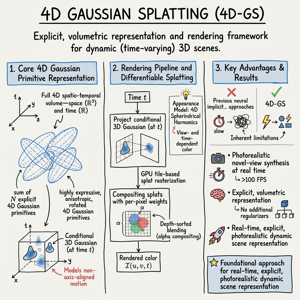
4D Gaussian Splatting (4D-GS) is an explicit, volumetric representation and rendering framework for dynamic (time-varying) 3D scenes. Introduced by Yang et al. (Yang et al., 2023), 4D-GS addresses the inherent limitations of previous neural implicit and deformable radiance field approaches by directly modeling the full 4D spatio-temporal volume—space (ℝ³) and time (ℝ)—with a set of highly expressive, anisotropic, rotated 4D Gaussian primitives. The method achieves photorealistic novel-view synthesis at real time, supporting diverse downstream applications in video-based scene capture, digital twins, interactive editing, and efficient dynamic view rendering.

1. Core 4D Gaussian Primitive Representation

A dynamic scene is encoded as a sum of $N$ explicit 4D Gaussian primitives $\{G_i\}$, each parameterized by a 4D mean $$\mu_i = (\mu_x, \mu_y, \mu_z, \mu_t) \in \mathbb{R}^4$$ and a full covariance $\Sigma_i \in \mathbb{R}^{4 \times 4}$: $$G_i(x, t) = \exp\!\left(-\frac{1}{2}\left( [x, t] - \mu_i \right)^\top \Sigma_i^{-1} \left( [x, t] - \mu_i \right) \right)$$ where $x \in \mathbb{R}^3$, $t \in \mathbb{R}$.

To enable stable optimization and full 4D anisotropy (including spatio-temporal orientation), $\Sigma_i$ is factored as: $\Sigma_i = R_i S_i^2 R_i^\top$ where $S_i = \mathrm{diag}(s_x, s_y, s_z, s_t)$ and $\{G_i\}$0 (a 4D rotation), parameterized using two quaternions. Each primitive thus defines an oriented, ellipsoidal support in space–time, with $\{G_i\}$1 controlling its temporal extent; $\{G_i\}$2 encodes its temporal position; and the full $\{G_i\}$3 enables modeling of non-axis-aligned motion (e.g., scene elements moving along oblique space–time paths).

Conditional and marginalization identities from multivariate Gaussians yield:

• The spatial “slice” at time $\{G_i\}$4 is a 3D Gaussian with:

$\{G_i\}$5

• The temporal marginal weight:

$\{G_i\}$6

2. Appearance Model: 4D Spherindrical Harmonics

View- and time-dependent color is modeled with a compact, explicit expansion: $\{G_i\}$7 where $\{G_i\}$8 are spherical camera directions and $\{G_i\}$9 is the 4D spherindrical basis: $$\mu_i = (\mu_x, \mu_y, \mu_z, \mu_t) \in \mathbb{R}^4$$0 for a scene duration $$\mu_i = (\mu_x, \mu_y, \mu_z, \mu_t) \in \mathbb{R}^4$$1, $$\mu_i = (\mu_x, \mu_y, \mu_z, \mu_t) \in \mathbb{R}^4$$2 being spherical harmonics.

This separable basis efficiently captures both high-frequency view-dependent reflectance and time-evolving appearance, with the learned coefficients $$\mu_i = (\mu_x, \mu_y, \mu_z, \mu_t) \in \mathbb{R}^4$$3 per Gaussian.

3. Rendering Pipeline and Differentiable Splatting

The rendered color $$\mu_i = (\mu_x, \mu_y, \mu_z, \mu_t) \in \mathbb{R}^4$$4 at pixel $$\mu_i = (\mu_x, \mu_y, \mu_z, \mu_t) \in \mathbb{R}^4$$5 and time $$\mu_i = (\mu_x, \mu_y, \mu_z, \mu_t) \in \mathbb{R}^4$$6 is computed by:

• Projecting each conditional 3D Gaussian (at $$\mu_i = (\mu_x, \mu_y, \mu_z, \mu_t) \in \mathbb{R}^4$$7) into image space using camera parameters, linearizing projection via the Jacobian $$\mu_i = (\mu_x, \mu_y, \mu_z, \mu_t) \in \mathbb{R}^4$$8.
• Computing the 2D projected Gaussian parameters:

$$\mu_i = (\mu_x, \mu_y, \mu_z, \mu_t) \in \mathbb{R}^4$$9

• Compositing splats with per-pixel weights:

$\Sigma_i \in \mathbb{R}^{4 \times 4}$0

where $\Sigma_i \in \mathbb{R}^{4 \times 4}$1 is a learned opacity.

GPU tile-based splat rasterization and depth-sorted blending (alpha compositing) yield efficient $\Sigma_i \in \mathbb{R}^{4 \times 4}$2 FPS rendering at high resolutions. Gaussians with negligible $\Sigma_i \in \mathbb{R}^{4 \times 4}$3 are pruned per frame.

4. Optimization and Training Protocol

Supervision is applied via photometric $\Sigma_i \in \mathbb{R}^{4 \times 4}$4 loss on (pixel, time) samples: $\Sigma_i \in \mathbb{R}^{4 \times 4}$5

Adaptive densification and pruning are performed using spatial/temporal gradient magnitudes:

• Gaussians with low spatial gradient are pruned (insufficient reconstruction).
• High-gradient Gaussians are split in full 4D space–time (to capture detail).
• The mean temporal gradient of $\Sigma_i \in \mathbb{R}^{4 \times 4}$6 is monitored to ensure even time coverage.

Training batches rays sampled uniformly in $\Sigma_i \in \mathbb{R}^{4 \times 4}$7, rather than sequential frames, enforcing temporal consistency and suppressing flicker.

Initialization uses colored point clouds (e.g., COLMAP) at $\Sigma_i \in \mathbb{R}^{4 \times 4}$8, with $\Sigma_i \in \mathbb{R}^{4 \times 4}$9 initialized randomly in $$G_i(x, t) = \exp\!\left(-\frac{1}{2}\left( [x, t] - \mu_i \right)^\top \Sigma_i^{-1} \left( [x, t] - \mu_i \right) \right)$$0 and temporal scale $$G_i(x, t) = \exp\!\left(-\frac{1}{2}\left( [x, t] - \mu_i \right)^\top \Sigma_i^{-1} \left( [x, t] - \mu_i \right) \right)$$1. End-to-end training runs for $$G_i(x, t) = \exp\!\left(-\frac{1}{2}\left( [x, t] - \mu_i \right)^\top \Sigma_i^{-1} \left( [x, t] - \mu_i \right) \right)$$2k iterations (batch size 4), with densification rate halved at halfway point.

5. Empirical Performance and Benchmarks

On the Plenoptic Video (multi-view, real) benchmark, 4D-GS achieves:

• PSNR = 32.01, DSSIM = 0.014, LPIPS = 0.055
• $$G_i(x, t) = \exp\!\left(-\frac{1}{2}\left( [x, t] - \mu_i \right)^\top \Sigma_i^{-1} \left( [x, t] - \mu_i \right) \right)$$3114 FPS on a single NVIDIA GPU

This surpasses prior neural dynamic scene models (DyNeRF, HexPlane, K-Planes, StreamRF, etc.) on both fidelity (PSNR, LPIPS) and real-time speed (often >10$$G_i(x, t) = \exp\!\left(-\frac{1}{2}\left( [x, t] - \mu_i \right)^\top \Sigma_i^{-1} \left( [x, t] - \mu_i \right) \right)$$4 faster than NeRF-based methods).

On monocular, under-constrained synthetic (D-NeRF) scenes, 4D-GS attains PSNR = 34.09 at real-time frame rates.

6. Methodological Distinctions and Theoretical Properties

• True 4D Native Representation: By representing spacetime as an explicit collection of 4D Gaussians, 4D-GS avoids overparametrizing time via separate deformation fields or per-frame duplication. All space–time correlations (motion, temporal occlusion, appearance drift) are encoded natively via the $$G_i(x, t) = \exp\!\left(-\frac{1}{2}\left( [x, t] - \mu_i \right)^\top \Sigma_i^{-1} \left( [x, t] - \mu_i \right) \right)$$5 and spherindrical expansion.
• Compact View-Time Appearance: Spherindrical harmonics provide a parsimonious but expressive basis for handling high-frequency view and time effects, enabling both photorealism and efficient memory use.
• Scalability and Flexibility: The rasterization and compositing algorithm is GPU-friendly and scales with the number of visible Gaussians per frame, not the number of input images or total scene length.
• Optimization Simplicity: No additional regularizers or motion priors are required. All geometry, appearance, and motion are learned end-to-end, with dynamic splitting and pruning providing automatic model adaptation.

7. Extensions and Applications

The 4DGS framework catalyzed further research exploring:

• Geometry-consistent extensions for sparse camera inputs by integrating multi-view stereo priors (Li et al., 28 Nov 2025).
• Aggressive model compression through pruning, quantization, and entropy-aware encoding to facilitate edge deployment (Wang et al., 11 Oct 2025, Zhang et al., 2024, Liu et al., 18 Mar 2025).
• Hybrid 3D–4D schemes to segregate static background (as pure 3D Gaussians) from dynamic elements (Oh et al., 19 May 2025).
• Generative content creation via diffusion-driven 4DGS pipelines (Ren et al., 2023).
• Real-time scene editing and semantic manipulation leveraging 4DGS’s explicit structure (Liu et al., 2 Oct 2025).
• Self-calibration from monocular video without external structure-from-motion (Li et al., 2024).

4D Gaussian Splatting has become a foundational approach for real-time, explicit, photorealistic dynamic scene representation, providing both practical utility and a mathematically tractable paradigm for space–time visual modeling (Yang et al., 2023, Yang et al., 2024).