Graph Neural Networks for Virtual Sensing in Complex Systems: Addressing Heterogeneous Temporal Dynamics

Abstract: Real-time condition monitoring is crucial for the reliable and efficient operation of complex systems. However, relying solely on physical sensors can be limited due to their cost, placement constraints, or inability to directly measure certain critical parameters. Virtual sensing addresses these limitations by leveraging readily available sensor data and system knowledge to estimate inaccessible parameters or infer system states. The increasing complexity of industrial systems necessitates deployments of sensors with diverse modalities to provide a comprehensive understanding of system states. These sensors capture data at varying frequencies to monitor both rapid and slowly varying system dynamics, as well as local and global state evolutions of the systems. This leads to heterogeneous temporal dynamics, which, particularly under varying operational end environmental conditions, pose a significant challenge for accurate virtual sensing. To address this, we propose a Heterogeneous Temporal Graph Neural Network (HTGNN) framework. HTGNN explicitly models signals from diverse sensors and integrates operating conditions into the model architecture. We evaluate HTGNN using two newly released datasets: a bearing dataset with diverse load conditions for bearing load prediction and a year-long simulated dataset for predicting bridge live loads. Our results demonstrate that HTGNN significantly outperforms established baseline methods in both tasks, particularly under highly varying operating conditions. These results highlight HTGNN's potential as a robust and accurate virtual sensing approach for complex systems, paving the way for improved monitoring, predictive maintenance, and enhanced system performance. Our code and data are available under https://github.com/EPFL-IMOS/htgnn.

• The paper introduces HTGNN, a framework that models heterogeneous sensor modalities and exogenous influences for improved virtual sensing.
• The paper employs a multi-component architecture, integrating a GRU-based encoder for low-frequency signals and a gated 1D-CNN for high-frequency dynamics.
• The paper demonstrates enhanced load prediction accuracy through case studies on bearing and bridge datasets, validating the robustness of the approach.

HTGNN: Addressing Heterogeneous Temporal Dynamics with Graph Neural Networks for Virtual Sensing

The paper introduces a Heterogeneous Temporal Graph Neural Network (HTGNN) designed for virtual sensing in complex systems, addressing the challenges posed by heterogeneous temporal dynamics and the influence of exogenous variables. HTGNN explicitly models signals from diverse sensors as distinct node types within a graph structure and integrates context from operating conditions, derived from exogenous variables, into the model architecture. The effectiveness of HTGNN is evaluated using two newly released, publicly available datasets: a test-rig bearing dataset and a comprehensive year-long simulated dataset for train-bridge-track interaction.

Addressing Limitations of Traditional Virtual Sensing

Traditional virtual sensing techniques often fall short in handling the complexities of real-world sensor data, particularly when dealing with heterogeneous sensor modalities and the diverse impact of exogenous variables. CNNs, while effective at capturing local patterns, struggle with long-range dependencies across different time scales. RNNs, designed for long-range temporal dependencies, may not effectively model high-frequency signals or extract localized features. Existing GNN approaches often assume that all nodes in the graph represent sensors with similar signal characteristics, failing to account for the diverse impact of exogenous variables on different sensor modalities. The resulting shifts in signal magnitude or frequency can lead to inaccurate predictions, particularly under varying operating conditions.

HTGNN Framework Overview

HTGNN addresses these limitations by explicitly modeling signals with distinct temporal dynamics as separate node types and incorporating operating condition context. The HTGNN architecture consists of four key components: Heterogeneous Temporal Graph Construction, Context-Aware Heterogeneous Dynamics Extraction, Heterogeneous Interaction Modeling, and Target Variable Inference.

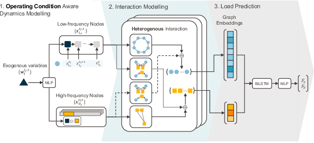
Figure 1: Architecture of the proposed Heterogeneous Temporal Graph Neural Network (HTGNN) for Load Prediction.

Heterogeneous Temporal Graph Construction

HTGNN employs a Heterogeneous Temporal Graph (HTG) to represent the sensor network, where nodes represent sensors and edges represent relationships between them. The graph consists of two types of nodes: low-frequency (L) nodes and high-frequency (H) nodes, with edges defined by the relationships between these node types (L-L, H-H, L-H, and H-L). This framework enables the HTG to capture and analyze the interactions and temporal evolution between low-frequency and high-frequency signals effectively.

Context-Aware Node Dynamics Extraction

HTGNN leverages context-aware dynamics extraction for each node, extending the strategy proposed in (Guo et al., 2024) to explicitly model shifts in both magnitude and frequency. Changes in exogenous variables, such as control inputs and environmental conditions, can significantly impact both the magnitude and the frequency characteristics of the sensor signals. The model extracts contextual information from exogenous variables using a Multi-Layer Perceptron (MLP) and integrates it into the dynamics modeling of both low-frequency and high-frequency sensor modalities using specialized techniques.

Encoding Low-Frequency Signals

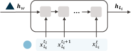
Figure 2: Architecture of a Gated Recurrent Unit (GRU)-based low-frequency signal encoder with exogenous variable encoding as the initial state.

Low-frequency signals are encoded using a Gated Recurrent Unit (GRU) network initialized with the exogenous variable encoding. This initialization allows the dynamics encoder to immediately integrate contextual information when processing the low-frequency signal sequence.

Encoding High-Frequency Signals

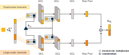
Figure 3: Architecture of a multi-scale Gated Convolutional Layers (GCLs)-based encoder for high-frequency signals, considering exogenous variable encoding as the gating signal.

To address shifts in high-frequency signals, the paper uses a 1D Gated Convolutional Neural Network (1D-GCNN). This model integrates a gating mechanism into the traditional 1D-CNN architecture, enabling dynamic adjustment of its frequency focus based on the operating context.

The core component of the 1D-GCNN is the Gated Convolutional Layer (GCL), which operates on an input sequence and the exogenous variable encoding, functioning as follows:

$$\begin{aligned} \mathbf{z}^t &= \text{Conv1D}(\mathbf{x}_i, \mathbf{W_z}) \ \mathbf{g}^t &= \sigma(\mathbf{W_g} \mathbf{h_w} + \mathbf{b_g}) \ \mathbf{o}^t &= \mathbf{z}^t \odot \mathbf{g}^t \end{aligned}$$

To accurately capture the multi-scale nature of high-frequency signals, the approach employs two parallel stacks of GCLs, each focusing on different temporal scales.

Heterogeneous Interaction Modeling

To effectively capture the complex relationships between sensor nodes and explicitly account for the influence of operating conditions on these interactions, the HTGNN model strategically models heterogeneous interactions within the temporal graph, including intra-modality interactions (homogeneous interactions among nodes with similar signal characteristics) and inter-modality interactions (across nodes with different signal characteristics).

Intra-modality Interactions

To effectively capture the interdependencies among sensors with similar frequency characteristics, Graph Convolutional Networks (GCNs) are employed. This enhances node representations by aggregating information from neighboring nodes that display correlated behaviors.

Inter-modality Interactions

To capture the influence of one signal type on another within the sensor network, Graph Attention Networks v2 (GATv2) are used. This approach enables dynamic computation of attention-weighted messages, allowing the model to dynamically assess the relevance of neighboring nodes based on their interactions.

Target Variable Inference

After extracting the context-aware dynamics from each node, these heterogeneous node representations are integrated to infer the target variable. First, the final node representations of both low-frequency and high-frequency nodes are flattened into a single input vector, which is then processed by a Bidirectional Long Short-Term Memory (BiLSTM) network. The final output of the BiLSTM is then passed through an MLP to generate the final prediction for the target variable.

Bearing Load Prediction Case Study

The paper assesses the applicability of the proposed HTGNN model for estimating bearing loads under various operating conditions, using data from temperature and vibration sensors. Data was collected at the SKF Sven Wingquist Test Centre (SWTC) using a face-to-face test rig with two identical single-row tapered roller bearings (TRBs) (Figure 4).

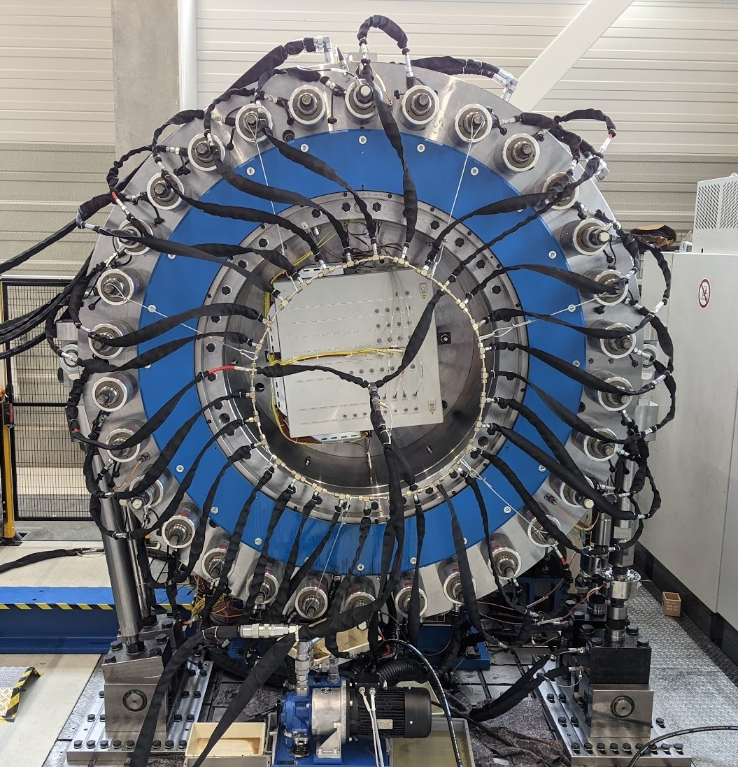
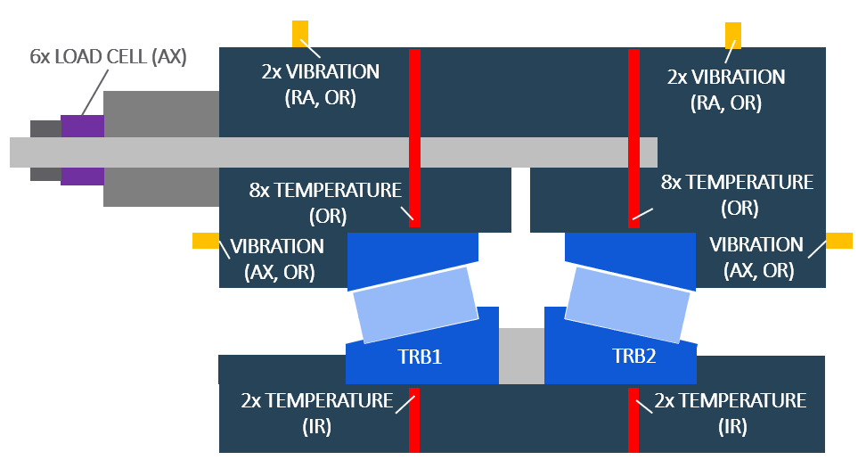
Figure 4: The SKF Sven Wingquist Test Centre (SWTC) TRB bearing test-rig (a) with sensor installation locations (b) for vibration, temperature, and load measurements.

The heterogeneous bearing graph is constructed with nodes representing sensors (temperature (T) and vibration (V)), modeling four types of relationships: T-T, V-V, T-V, and V-T (Figure 5).

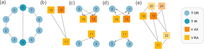
Figure 5: Heterogeneous graphs for bearing sensor network relationship modeling. (a) Temperature-Temperature (b) Vibration-Vibration (c) Temperature-Vibration (d) Vibration-Temperature (e) Connectivity across two test rig bearings (the connectivity between T nodes omitted for simplicity).

The results demonstrate that HTGNN's architecture, which explicitly models heterogeneous relationships and their dependence on operating conditions, enables it to effectively extract information from both temperature and vibration sensors across varying rotational speeds, resulting in improved load prediction.

Bridge Load Prediction Case Study

The paper evaluates the proposed HTGNN model for bridge health monitoring, specifically focusing on estimating live load on the bridge deck from displacement and acceleration signals.

Raw simulation data was first cropped to focus on the period when the train was fully on the bridge based on the magnitude of the displacement sensors. To simulate realistic sensor noise, additive white Gaussian noise with a signal-to-noise ratio (SNR) of 35 dB was introduced. Finally, the dataset was divided into windows with a length of 60 samples (0.6 seconds at 100 Hz) and a stride of 5. The heterogeneous bridge graph is constructed following the same principles established for the bearing graph, with nodes representing displacement (D) and acceleration (A) sensors and modeling four types of relationships: D-D, A-A, D-A, and A-D.

Experimental Results and Ablation Study

The experimental results demonstrate that HTGNN consistently exhibits competitive performance across all temperature ranges, showing particular strength at lower temperatures. The ablation study highlights the importance of key design choices in HTGNN: explicit modeling of exogenous variables (operating conditions) and differentiated node and edge types for effective fusion of heterogeneous sensor information (Figure 6).

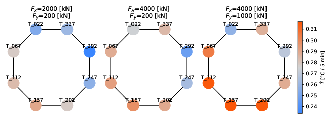
Figure 6: Temperature change rates at different bearing locations under varying axial ($F_x$) and radial ($F_y$) load conditions and a constant rotational speed (30 [r/min]).

Conclusion

The HTGNN framework effectively addresses the challenges of heterogeneous temporal dynamics and varying operating conditions in complex systems. The framework's ability to explicitly model the complex, heterogeneous relationships between sensor modalities and its capacity to extract operating condition-aware dynamics enable it to adapt to changing operating conditions and accurately predict loads even in scenarios where traditional methods struggle. The consistent robustness and accuracy of HTGNN in both case studies highlight its potential as a reliable virtual sensor for diverse IIoT applications, enabling effective monitoring, predictive maintenance, and enhanced system performance.