Measuring Cometary Nuclei Behind Bright Comae: PSF Delta Decomposition with Bicubic Resampling and an Application to Interstellar Comet 3I/ATLAS C/2025 N1
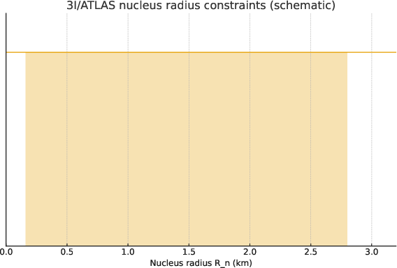
Abstract: Measuring cometary nuclei is notoriously difficult because they are usually unresolved and embedded within bright comae, which hampers direct size measurements even with space telescopes. We present a practical, instrumental method that, stabilises the inner core through bicubic resampling, performs forward point-spread function PSF+convolution, and separates the unresolved nucleus from the inner-coma profile via an explicit Dirac Delta function added to a Rho-1 surface brightness law. The method yields the nucleus flux by fitting an azimuthal averaged profile with two amplitudes only PSF core and convolved coma, with transparent residual diagnostics. As a case study, we apply the workflow to the interstellar comet 3I/ATLAS alias C/2025 N1, incorporating Hubble Space Telescope constraints on the nucleus size. We find that radius solutions consistent with 0.16 <= Rn <= 2.8 km for Pv = 0.04 are naturally recovered, in line with the most recent HST upper limits. The approach is well-suited for survey pipelines Rubin LSST and targeted follow up.

Paper Prompts
Sign up for free to create and run prompts on this paper using GPT-5.
Top Community Prompts
Explain it Like I'm 14
Overview
This paper is about a clever way to measure the size of a comet’s solid core (called the “nucleus”) even when it’s hidden behind the comet’s bright fuzzy cloud of gas and dust (the “coma”). The authors show a simple, practical technique that separates the tiny, point-like light from the nucleus from the wider glow of the coma in real telescope images. They then try it on an especially interesting object: 3I/ATLAS, an interstellar comet that came from outside our solar system.
What questions were the researchers trying to answer?
They wanted to answer two main questions:
- How can we reliably measure the brightness (and therefore size) of a comet’s nucleus when it’s drowned out by the bright coma and blurred by the telescope’s optics?
- Does this method match what space telescopes like Hubble suggest about the size of 3I/ATLAS’s nucleus?
How did they do it? (Methods explained simply)
Think of trying to spot a firefly right next to a bright streetlamp. The lamp’s glow makes the firefly hard to see. In comet images, the streetlamp glow is the coma, and the firefly is the nucleus.
Two key ideas make their method work:
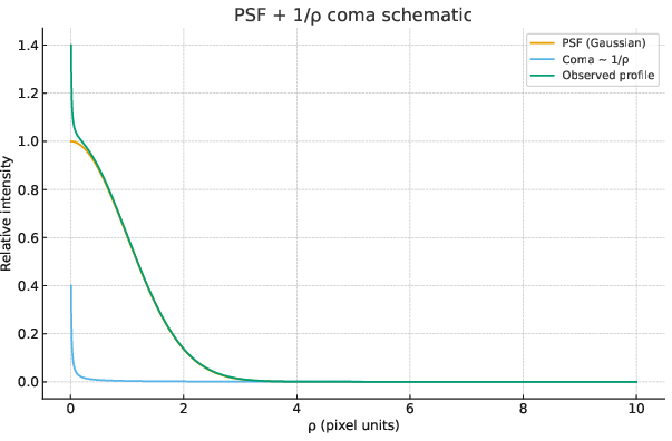
- The “camera blur” model (PSF)
- Any camera or telescope blurs light a little. The pattern of blur is called the point-spread function, or PSF.
- If the nucleus is too small to resolve, it looks like a point source blurred exactly by this PSF.
- The coma is bigger and spreads out more, so its light looks smoother and broader.
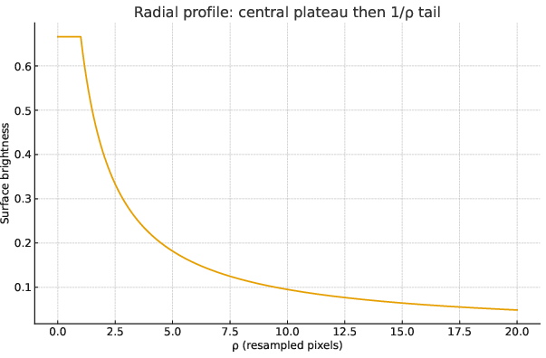
- A simple brightness recipe for the inner coma
- Near the center, the coma’s surface brightness falls off roughly like 1 divided by the distance from the center (written as “1/ρ”).
- The nucleus is modeled as a perfect point (mathematically a “delta function”), which after blur looks just like the PSF.
- The observed image, then, is “PSF from the nucleus” plus “blurred 1/ρ coma.”
To make the measurement more stable, they do two practical steps:
- Bicubic resampling: They “zoom in” on the center of the image by breaking each pixel into smaller pixels (4×4). This makes the central profile smoother, reduces pixel alignment quirks, and helps separate the sharp core (nucleus) from the broader tail (coma), while keeping total brightness the same.
- Azimuthal averaging: They average the image brightness in circles around the center. This turns the complicated 2D picture into a simple 1D curve: brightness vs. distance from the center. That curve is easier to fit.
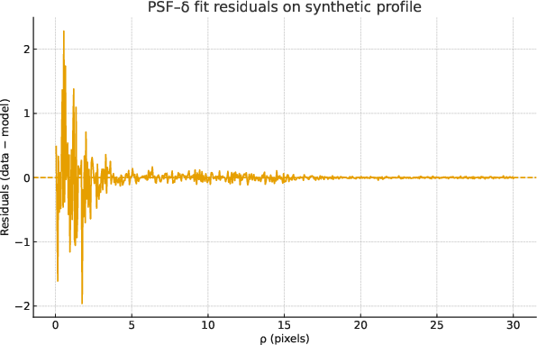
Finally, they “fit” that curve using only two amplitudes:
- One for the PSF-shaped core (the nucleus brightness).
- One for the blurred 1/ρ tail (the coma brightness).
From the fitted nucleus brightness, they use standard astronomy formulas to get a magnitude and then estimate the nucleus size. This needs an assumption about how reflective the surface is (the “albedo,” often around 4% for dark comet material).
What did they find, and why does it matter?
Main results:
- The method recovers nucleus sizes in the range that Hubble Space Telescope (HST) suggests for 3I/ATLAS. Assuming a typical dark comet surface (albedo p_V ≈ 0.04), they find radii between about 0.16 km and 2.8 km are consistent with the data.
- In a worked example using typical observing numbers, the method gives a radius around 0.31 km, which fits within HST’s limits.
Why it’s important:
- Measuring comet nuclei is hard because the coma hides them and they’re too small to resolve. This method gives a practical, transparent way to tease out the nucleus signal without requiring fancy, heavy computations.
- It’s well-suited for big survey projects (like Rubin/LSST) that will collect tons of comet images and need fast, consistent measurements.
- For interstellar comets like 3I/ATLAS, knowing the nucleus size helps us compare them to comets from our own solar system and learn how small bodies form in other star systems.
What could this mean going forward? (Implications)
- Better pipelines: Observatories can plug this method into their processing to quickly estimate nucleus sizes or set upper limits when the nucleus is too faint to see clearly.
- More reliable measurements: By modeling both the sharp core and broad coma together, the method reduces the risk of mixing them up and getting biased results.
- Focus on the big unknowns: The biggest source of uncertainty is how reflective the nucleus is (albedo). If future missions or observations can improve albedo estimates, nucleus size measurements will become much more precise.
- Interstellar insights: Applying this to interstellar comets helps us compare their building blocks to ours, giving clues about how planets and small bodies form across the galaxy.
Knowledge Gaps
Knowledge gaps, limitations, and open questions
Below is a concise list of unresolved issues and concrete next steps that the paper leaves open for future research.
- Validate on real, non-synthetic data: Demonstrate the PSF–delta decomposition on actual images of 3I/ATLAS (and other comets) with full data release, rather than synthetic profiles and a single worked example with ad hoc numbers (e.g., D0_rec, D1_mediana).
- PSF identifiability and degeneracy: Quantify the bias and variance in recovered nucleus amplitude A when PSF width/shape is not perfectly known; provide identifiability conditions and simulations across seeing, SNR, and pixel scale.
- PSF mismatch in non-sidereal tracking: Address the mismatch between comet PSF (non-sidereal tracked) and field-star PSF (trailed) used for empirical PSF estimation; develop comet-specific PSF-building or trailing-PSF models.
- Chromatic and spatial PSF variability: Evaluate impact of color differences (red comet vs stars), atmospheric dispersion, field-dependent PSF, and temporal PSF changes on A and B; propose corrections or calibration strategies.
- PSF wings and scattered light: Quantify sensitivity of A to PSF wing uncertainties and optical scattering halos, especially in bright comae; include wing-parameter priors or regularization in the fit.
- Bicubic resampling biases: Provide a quantitative assessment of how 4×4 bicubic resampling alters noise properties, induces pixel correlations, and biases A; compare against alternatives (e.g., drizzling, FFT super-resolution) and justify the choice of s=4.
- Coma model generality: Extend beyond a fixed ρ⁻¹ surface-brightness law; fit the inner-coma slope (e.g., ρ⁻γ), broken power-laws, or physically motivated models (finite grain lifetimes, acceleration, radiation pressure) and assess changes in A.
- Central divergence handling: Specify and test inner cutoff/regularization for the ρ⁻¹ model near ρ→0 to prevent divergence in the convolution; quantify its effect on A and residuals.
- 2D anisotropy treatment: Move beyond azimuthal averaging and masking to explicitly model jets/fans and azimuthal asymmetries (e.g., sector-based fits or full 2D forward models) to avoid bias in A.
- Trailing and motion blur: Incorporate exposure-time trailing and motion blur into the forward model (convolve with a trail kernel) and evaluate its impact on A under typical survey conditions.
- Aperture selection and core size: Provide objective criteria for choosing the inner N×N region used for resampling and fitting; quantify sensitivity of A to this choice.
- Background and blending systematics: Develop robust strategies for sky-background estimation in the presence of extended coma, gradients, and field-star blending; measure the induced bias on A.
- Photometric calibration under color terms: Assess calibration biases due to color differences (comet vs standard stars) and filter bandpasses; provide S-corrections or color-term models for m and H.
- Phase function assumptions: Test different nucleus phase functions (non-linear, Hapke-like) and quantify the sensitivity of H—and thus Rn—to the adopted β and Φ(α), especially at large phase angles.
- Albedo degeneracy: Provide a pathway to constrain pV (e.g., thermal IR, polarimetry, multiband photometry) and quantify how better pV priors reduce σR; explore interstellar comet albedo plausibility ranges.
- Error model completeness: Include correlated noise from resampling, PSF-fit covariance between A and PSF parameters, and sky/coma uncertainties in σA; report full covariance matrices from the fit.
- Goodness-of-fit and model selection: Complement residual plots with quantitative metrics (χ², AIC/BIC, cross-validation) to detect model inadequacy (PSF mismatch, wrong coma slope) and avoid overfitting.
- Upper-limit methodology under non-uniform noise: Generalize the matched-filter upper-limit calculation to spatially varying noise dominated by residual coma; demonstrate on real nondetections.
- Reproducibility and code availability: Release open-source code, test datasets, and configuration files to enable independent replication and benchmarking across instruments and observing conditions.
- Survey pipeline readiness: Benchmark runtime, memory, and failure modes in Rubin/LSST-like pipelines; define automatic masking of anisotropies and quality-control flags for operational deployment.
- Saturation and detector nonlinearity: Address how near-core saturation, blooming, or nonlinearity affect A and the PSF fit; define detection thresholds and correction procedures.
- Multi-epoch variability: Explore temporal variability (rotation, activity changes) and its effect on A; propose multi-epoch joint fitting strategies to track nucleus flux across changing comae.
- Multi-band joint modeling: Combine bands to separate dust color and nucleus reflectance; co-fit A across filters with coupled PSF and coma models to reduce degeneracies.
- Validation against alternative methods: Compare PSF–delta decomposition with deconvolution (e.g., Richardson–Lucy), coma extrapolation, and synthetic injection/recovery tests to quantify relative performance.
- Applicability across geometries: Test method robustness across heliocentric distances, phase angles, and activity levels; define the parameter space (seeing, SNR, pixel scale) where A is reliably recoverable.
Practical Applications
Immediate Applications
The paper introduces a lightweight PSF–delta decomposition with bicubic resampling that separates unresolved comet nuclei from bright inner comae via a two-parameter fit. The following are actionable uses that can be deployed now:
- Stronger moving-target photometry in survey and follow-up pipelines
- Sector: software, astronomy/observatories (e.g., Rubin/LSST, Pan-STARRS, ZTF), robotics (autonomous observatories)
- What: Add a “nucleus flux extractor” step that azimuthally averages the inner profile, fits A·PSF + B·(ρ⁻¹∗PSF), and outputs nucleus flux or an upper limit with residual diagnostics.
- Tools/workflows: Python/Astropy-Photutils module; plugin for the LSST Science Pipelines; Jupyter notebooks for batch processing FITS frames; optional wrappers for SExtractor/SEP outputs.
- Dependencies/assumptions: Accurate empirical PSF from field stars near the comet; coma close to ρ⁻¹ in the fitted core; sufficient SNR; detector linearity; proper non-sidereal tracking and de-trailing for PSF stars; stable photometric zero points.
- Automated upper limits for non-detections using matched filtering
- Sector: observatories, academia, proposal support
- What: Implement the paper’s matched-filter PSF-fit SNR and A_UL calculation to produce robust nucleus radius limits even when the nucleus is not detected.
- Tools/workflows: Add a “non-detection UL” button in observatory QA dashboards; web calculator that ingests PSF, core-noise estimate, and exposure metadata.
- Dependencies/assumptions: Noise characterization in the PSF-fit core; valid PSF sampling on the resampled grid; approximate noise uniformity or per-pixel noise map.
- Observation planning and exposure-time calculators for comets
- Sector: observatories, mission planning, education
- What: Use the forward model to forecast detectable nucleus amplitudes A (or ULs) vs. exposure time, seeing, and pixel scale; optimize cadence and depth.
- Tools/workflows: ETC add-ons that accept a PSF FWHM, expected coma normalization, and desired nucleus size threshold.
- Dependencies/assumptions: Forecasts require plausible coma ρ⁻¹ normalization (B), realistic seeing and PSF wings, and target ephemerides.
- Rapid follow-up triage for interstellar objects and active asteroids
- Sector: survey ops, time-allocation committees, planetary defense science
- What: Convert quick-look images into nucleus size estimates/limits to decide whether deeper observations or spectroscopy are warranted.
- Tools/workflows: Real-time notebooks or Kafka consumers on alert streams that compute A, B, diagnostics and post a triage score.
- Dependencies/assumptions: Timely PSF star sampling in the same exposure or field; standardized calibration frames; known or assumed phase functions.
- Archival reprocessing to build nucleus-size and upper-limit catalogs
- Sector: academia, data centers, meta-analyses
- What: Apply the method to past comet images (including HST and ground-based data) to generate a uniform catalog of nucleus fluxes and limits with uncertainty propagation.
- Tools/workflows: Batch processing scripts over archives (e.g., MAST, NOIRLab Astro Data Lab); a results schema including A, B, fit residuals, and QA flags.
- Dependencies/assumptions: Archival PSF reconstruction (or analytic PSFs with characterized wings); consistent zero-point metadata; deblending of nearby stars.
- Improved spectroscopic aperture corrections and continuum subtraction
- Sector: spectroscopy (telescopes/instruments), academia
- What: Use the derived nucleus-to-coma flux partition to correct slit/aperture contamination, improving gas/dust production-rate inferences.
- Tools/workflows: Pipeline hook that ingests photometric decomposition and applies wavelength-appropriate corrections to spectra.
- Dependencies/assumptions: Temporal proximity between imaging and spectroscopy; filter-to-slit throughput mapping; coma color gradients are small over the bandpass.
- PSF QA and seeing diagnostics for moving-target imaging
- Sector: observatory operations, instrumentation
- What: Use core residual patterns and “central-plateau width vs seeing” relations to flag PSF mismatch, guiding focus/seeing assessments and PSF model choice.
- Tools/workflows: Residual dashboards; notifications when core residuals exceed thresholds.
- Dependencies/assumptions: Sufficient star counts for PSF characterization; stable guiding/tracking; bicubic resampling preserves flux and doesn’t introduce artifacts.
- Pro–am and education kits for comet nucleus photometry
- Sector: education, citizen science, amateur astronomy
- What: Provide ready-to-run notebooks and tutorials to let advanced amateurs apply the method to backyard CCD data, contributing to pro–am campaigns.
- Tools/workflows: Open-source notebooks, sample data, and a step-by-step checklist (bias/flat, resampling, PSF, fit, uncertainty).
- Dependencies/assumptions: Reasonable seeing relative to pixel scale; enough field stars for empirical PSF; adoption of standardized calibration practices.
Long-Term Applications
These applications need scaling, integration, or additional research before broad deployment:
- Real-time nucleus-size estimates in survey alert packets
- Sector: survey ecosystems (Rubin/LSST brokers), software
- What: Embed nucleus flux fractions and radius posteriors (with albedo priors) into moving-object alerts for automated science triage.
- Tools/workflows: Broker plugins that run decomposition on difference or direct images, publish A, B, QA flags, and upper limits.
- Dependencies/assumptions: Low-latency PSF modeling at alert scale; reliable moving-target photometry in crowded fields; robust handling of anisotropic comae.
- Population studies of comet and interstellar-object nuclei
- Sector: academia, agencies
- What: Aggregate uniform A/B decompositions across surveys to constrain size distributions, activity scaling, and formation histories.
- Tools/workflows: Bayesian hierarchical models that fold in albedo and phase-law uncertainties; cross-matching thermal IR to break albedo–size degeneracy.
- Dependencies/assumptions: Consistent cross-survey calibration; representative albedo priors per dynamical class; multiwavelength coverage.
- Mission and instrument target selection
- Sector: space agencies, industry (mission design)
- What: Use early size estimates/limits to prioritize flyby/ rendezvous targets (e.g., very small or unusually large nuclei), and to refine instrument exposure budgets.
- Tools/workflows: Integration into mission planning toolchains (SPICE, exposure planners) and target ranking dashboards.
- Dependencies/assumptions: Early-time photometry with adequate SNR; vetted phase functions for conversion to size; coordination with thermal measurements.
- Adaptive scheduling for robotic telescope networks
- Sector: robotics, observatory ops
- What: Use residual diagnostics and SNR forecasts to adapt exposure times and filter choices on the fly for moving targets under variable seeing.
- Tools/workflows: Scheduler feedback loops that ingest fit quality, predicted A_UL, and PSF mismatch scores.
- Dependencies/assumptions: Real-time PSF estimation; robust failure modes when jets/fans invalidate ρ⁻¹ assumptions; latency budgets.
- ML-assisted detection of coma anisotropies and PSF mismatch
- Sector: software, academia
- What: Train models on residual maps to automatically flag jets/fans and trigger 2D anisotropic coma models when the spherical ρ⁻¹ law breaks down.
- Tools/workflows: CNNs or U-Nets trained on simulated and labeled residuals; integration with the two-parameter fit as a first-pass filter.
- Dependencies/assumptions: Curated training sets; explainability requirements for survey QA; avoidance of overfitting in low-SNR regimes.
- Instrument and camera design guidance for moving-target science
- Sector: industry (detectors/optics), observatories
- What: Use sensitivity of decomposition to PSF wings and pixel phase to derive requirements for pixel scale, PSF stability, and baffling.
- Tools/workflows: End-to-end simulations of A/B recoverability vs. PSF wings and sampling; design trades for future comet-focused instruments.
- Dependencies/assumptions: Validated forward models for specific optical trains; realistic sky backgrounds and tracking jitter models.
- Standardized public API and registry for nucleus-size estimates
- Sector: data infrastructure, agencies
- What: A community service that ingests images/metadata and returns nucleus flux, radius posteriors, and upper limits with provenance and QA, building a global registry.
- Tools/workflows: Cloud microservices; DOI-minted result objects; interoperability with MPC and NASA archives.
- Dependencies/assumptions: Agreement on metadata schemas; authentication and data-rights policies; compute/storage funding.
- Joint optical–thermal inversion to reduce albedo/phase uncertainty
- Sector: academia, agencies
- What: Combine optical A-estimates with thermal IR (e.g., NEOWISE, JWST/MIRI) to solve for both R and pV, reducing dominant uncertainties.
- Tools/workflows: Coupled thermophysical models; cross-calibrated photometry pipelines; joint posterior sampling.
- Dependencies/assumptions: Temporal proximity of observations; knowledge of thermal inertia and beaming parameters; consistent absolute calibration.
- Generalization to other core+halo astrophysical systems
- Sector: academia
- What: Adapt the PSF–delta + convolved-profile framework to active asteroids, Centaurs, or other unresolved-core plus power-law halo targets; exploratory applications to AGN core/host separation at low SNR.
- Tools/workflows: Replace ρ⁻¹ with appropriate surface-brightness laws; extend to 2D anisotropic kernels.
- Dependencies/assumptions: Valid physics for alternative halos; careful PSF wing characterization; control of deblending in crowded fields.
Glossary
- Absolute magnitude: Brightness standardized to 1 au from the Sun and observer and zero phase angle. "The absolute magnitude is"
- Astrometric calibration: Aligning image coordinates to the celestial reference frame. "Bias/flat correction, cosmic-ray cleaning; astrometric/photometric calibration."
- Azimuthal asymmetries (jets/fans): Non-circular features in the coma indicating directional activity. "azimuthal asymmetries (jets/fans) indicating breakdown of spherical symmetry."
- Azimuthal averaging: Averaging intensity in circular annuli to produce a radial profile. "After azimuthal averaging,"
- Bicubic resampling: Upsampling using bicubic interpolation to mitigate pixel-phase systematics while conserving flux. "stabilises the inner core through bicubic resampling,"
- Coma: The diffuse envelope of gas and dust surrounding a comet’s nucleus. "separates the unresolved nucleus from the inner-coma profile"
- Convolution: Blending a model with the PSF to simulate observational blurring. "performs forward point-spread function (PSF)+convolution,"
- Dirac delta (2D): A two-dimensional impulse function representing a point source. "where is the unresolved nucleus flux, is the 2D Dirac delta,"
- Effective diameter: The equivalent spherical diameter inferred from brightness and albedo. "Assuming geometric albedo , the effective diameter is ~km"
- Effective number of pixels: The PSF-dependent pixel count relevant for noise in matched filtering. "where is the effective number of pixels for the PSF on the chosen grid."
- Empirical PSF: A PSF measured from field stars rather than assumed analytically. "Empirical PSF estimation from field stars (or analytic PSF if needed)."
- Forward model: Predicting observed data by simulating instrumental effects from intrinsic sources. "Forward model in 2D"
- Full width at half maximum (FWHM): A measure of PSF width at half of its maximum. "The central-plateau width scales with the assumed PSF FWHM,"
- Geocentric distance: Distance from Earth to the object, in astronomical units. "geocentric distance (au)"
- Geometric albedo: The fraction of incident light reflected by the surface. "Assuming geometric albedo ,"
- Heliocentric distance: Distance from the Sun to the object, in astronomical units. "heliocentric distance (au)"
- Hubble Space Telescope (HST): A space telescope providing high-resolution observations. "HST observations place the nucleus diameter between ~km and ~km"
- Matched-filter: An optimal detection technique weighting data by the PSF to maximize SNR. "For a matched-filter (PSF-fit) estimator, the signal-to-noise ratio (SNR) for a point source with amplitude is"
- Moffat (PSF): A PSF model with power-law wings used in astronomy. "Given an empirical or analytic PSF (Gaussian/Moffat)"
- Perihelion: The point in an orbit closest to the Sun. "as the comet approaches perihelion"
- Phase function: The dependence of brightness on solar phase angle. "and phase function ."
- Photometric calibration: Converting instrumental counts to physical magnitudes. "Photometric calibration and radius inference"
- Photometric zero point: The magnitude corresponding to one count per second. "With photometric zero point (mag for 1 count s)"
- Pixel-phase effects: Flux variations due to sub-pixel source positioning. "explicit treatment of the instrumental PSF and pixel-phase effects."
- Point-spread function (PSF): The instrument’s response to a point source, which blurs images. "point-spread function (PSF)"
- Poisson statistics: Shot-noise model where variance equals the mean count. "If we adopt Poisson statistics on as a lower bound"
- Rubin/LSST: The Vera C. Rubin Observatory’s Legacy Survey of Space and Time. "well-suited for survey pipelines (e.g. Rubin/LSST)"
- Seeing: Atmospheric blurring affecting image quality. "inner-plateau width vs.\ seeing,"
- Signal-to-noise ratio (SNR): A measure of detection significance relative to noise. "the signal-to-noise ratio (SNR) for a point source with amplitude is"
- Surface brightness: Brightness per unit angular area on the sky. "a surface-brightness law."
- Upper limit (non-detection): A bound on source flux when a detection is not significant. "Upper-limit (non-detection) estimate"
- Weighted least squares: Fitting that accounts for varying measurement uncertainties. "fit Eq.~(\ref{eq:model}) to the azimuthally averaged profile via weighted least squares"
- PSF wings: The extended low-level parts of the PSF that can bias measurements. "The dominant systematics are PSF wings, coma anisotropy, and albedo uncertainty."
Collections
Sign up for free to add this paper to one or more collections.