On early-warning of full versus partial Atlantic overturning circulation collapse
Abstract: Climate models indicate a possible collapse of the Atlantic Meridional Overturning Circulation (AMOC) even for moderate climate change scenarios. There is considerable uncertainty in its likelihood for a given scenario and the critical global warming threshold. An alternative are early-warning signals (EWS) in AMOC fingerprints, which leverage generic statistical properties before destabilization of a steady state (a saddle-node bifurcation). But an AMOC collapse may be a sequence of partial collapses with shutdown of deep water formation in distinct regions. A conceptual model is presented featuring a sequential shutdown in two deep water formation regions. Multiple tipping points are present that do not follow the saddle-node normal form. As a result, the choice of the observable used to monitor EWS dramatically influences the prediction of the collapse via EWS. Various trends in EWS for different observables make it hard to determine what type of collapse (partial or full) will follow.
Paper Prompts
Sign up for free to create and run prompts on this paper using GPT-5.
Top Community Prompts
Explain it Like I'm 14
What is this paper about?
This paper looks at a big ocean current called the Atlantic Meridional Overturning Circulation (AMOC). You can think of the AMOC like a giant conveyor belt moving warm water north and cold water south in the Atlantic Ocean. If this conveyor belt slows down or stops, it could seriously change weather patterns, especially in Europe.
The authors ask: Can we spot early warning signs before the AMOC collapses? And if we do see warnings, can we tell whether the collapse will be partial (only some parts shut down) or full (the whole thing shuts down)?
What questions did the researchers ask?
The paper focuses on simple versions of these big questions:
- Are there early warning signals that show the AMOC is getting close to a collapse?
- Do those warning signs look different depending on whether the collapse is partial or full?
- Does it matter what exactly we measure (which “observable” we watch) when we look for warning signs?
- Can we use those warning signs to predict when a collapse will happen?
How did they study it?
The author uses a small, simplified model (also called a “conceptual model”) of the Atlantic to test how warning signals behave. This helps avoid some of the big uncertainties in huge climate models and real-world data.
A simple picture: a ball in a bowl
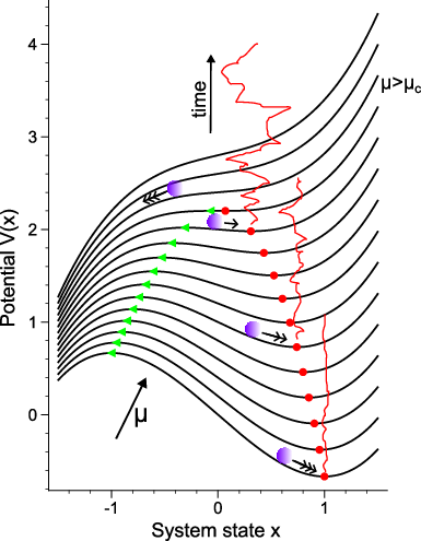
Imagine a ball resting in the bottom of a bowl. Small nudges (like random weather wiggles) push the ball around, but it rolls back to the bottom. As the system gets less stable (closer to a “tipping point”), the bowl gets flatter. The same nudges now push the ball farther, and it takes longer to roll back. That’s called “critical slowing down.” We can detect it by looking for:
- Bigger swings (higher variance)
- Longer memory (higher autocorrelation), meaning each wiggle looks more like the last one
These changes are called early-warning signals.
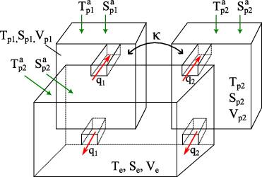
The model: three boxes and two northern regions
To capture the main idea without too much detail, the model uses three “boxes” of ocean water:
- One big equatorial box (the warm, central Atlantic)
- Two northern boxes (the colder regions where deep water forms), representing:
- The Labrador–Irminger Seas
- The Nordic Seas
Water moves between these boxes based on differences in temperature and saltiness (which control density). The “flow” between boxes is stronger when the density difference is larger.
The model lets the two northern boxes be different:
- One might get more freshwater (from melting ice or rain), which makes it less salty and lighter
- One might cool more, which makes it denser and helps deep water formation
By changing these conditions, the model can produce:
- An “ON” state (modern AMOC working)
- A “PC” state (partially collapsed; one northern region shuts down while the other still works)
- An “OFF” state (fully collapsed; both shut down)
Early-warning signals explained
To mimic weather and other random changes, the model adds small random “wiggles” (noise). The author checks different ways of measuring the system (different “observables”), such as:
- The overall AMOC strength (think: the conveyor belt speed)
- The local flows to each northern box
- Simple combinations of temperature and salinity in each box (like “T + S”)
Then the paper looks at how the variance and autocorrelation of these measurements change as the system gets closer to a tipping point.
What did they find?
Here are the main takeaways:
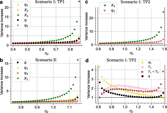
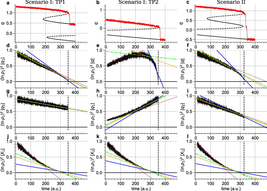
- Warning signals depend a lot on what you measure. Some measurements show strong warnings; others show almost nothing, even when the system is close to collapse. For example, “T + S” in the region that’s about to tip often gives clearer signals than the overall AMOC strength.
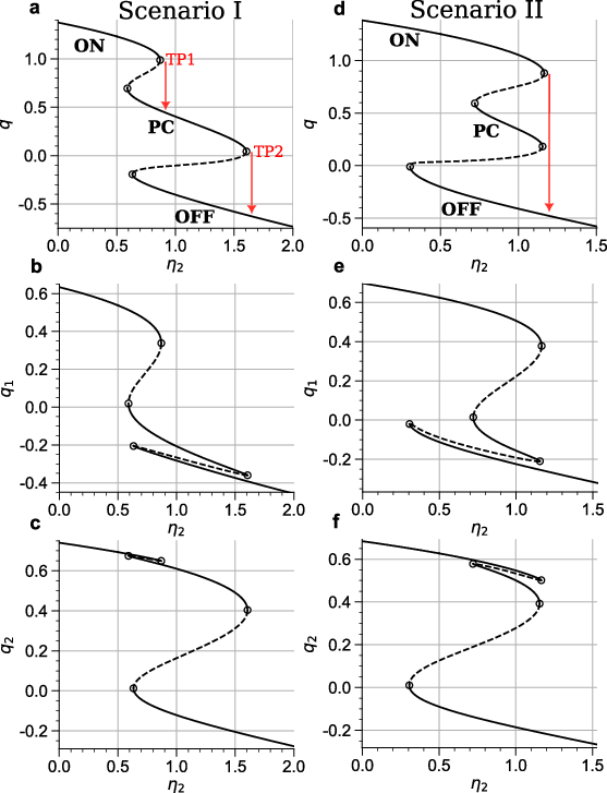
- The AMOC might collapse in steps. In one scenario, one northern region shuts down first (partial collapse), and only later the other shuts down (full collapse). In another scenario, the AMOC jumps straight from ON to OFF.
- Warning signals can be confusing. They don’t always increase smoothly. On a branch that’s “close to tipping” on both sides, signals can go up in one direction and down in the other, or even rise and fall in a wiggly way. This makes it hard to say “we are definitely getting closer to a collapse” just from a single trend.
- Predicting “when” is tricky and can be biased. Some methods try to predict the time of tipping by assuming a standard pattern (a “normal form”) for how the system slows down. But real systems and many observables don’t follow that pattern until very close to the tipping point. That means predictions can be too early or too late depending on which measurement you use.
- Local versus global signals: Watching measurements only from the “wrong” region can miss the warning signs, even when the whole AMOC is about to fail. In other words, where you look matters.
Why does this matter?
If the AMOC collapses, it could cause:
- Cooling in Northern Europe
- Warming in the Southern Hemisphere
- Changes in rain, storms, and ecosystems
Because collapse might be sudden and hard to reverse, we want warning signs in advance. This paper shows that:
- We must choose the right things to measure
- We need multiple indicators, not just one
- We shouldn’t assume simple rules for predicting the time of tipping
In short, early-warning signals are useful but can be misleading if we don’t understand what’s being measured and how the system really behaves.
Simple final takeaway
The AMOC is like a giant ocean conveyor belt that could slow down or stop. Warning signs exist, but they depend strongly on what and where we measure. Collapse can happen in steps or all at once, and the signals can be messy. That means we need smarter, carefully chosen indicators and better understanding before we trust predictions of when a collapse might happen.
Knowledge Gaps
Knowledge gaps, limitations, and open questions
Below is a consolidated list of what remains uncertain or unexplored, framed to guide concrete next steps for future research.
- Empirical validation across model hierarchies
- No systematic test that the paper’s key EWS behaviors (observable dependence, non-monotonic trends, concave/convex λ-scaling, masking of EWS in AMOC strength) occur in state-of-the-art coupled or eddy-resolving models under realistic forcing histories.
- Lack of a multi-model intercomparison using identical EWS workflows to quantify robustness and model spread in partial vs full collapse pathways and in the performance of different observables.
- Mapping conceptual parameters to the real ocean
- Unclear how box-model heterogeneity parameters (δT, δS), coupling (κ), and volume ratio (ω) map quantitatively to present-day atmospheric/oceanic boundary conditions and observed regional fluxes.
- No inverse-calibration framework to infer δT, δS, κ from observations and reanalyses (e.g., mixed-layer heat/freshwater budgets in Labrador–Irminger vs Nordic seas).
- Sensitivity surfaces and bifurcation topology across the full parameter space (η1, η2, η3, κ, ω, δT, δS) are not charted; regions where partial collapse is structurally stable remain unquantified.
- Observables: identification, measurability, and deployment
- The “special” observables aligned with the edge-state direction (e.g., X1 ≡ T1+S1 spiciness-like) are not operationalized for real data: how to construct robust, monitorable T+S indices with sparse, heterogeneous sampling and changing observing systems (RAPID/OSNAP/Argo/altimetry)?
- No procedure is given to discover optimal observables from data in high-dimensional models (e.g., Koopman/transfer-operator eigenfunctions, dynamic mode decomposition, or supervised dimension reduction targeting the slow mode).
- Open question whether density-gradient/AMOC-strength proxies can be systematically corrected to recover EWS when they poorly project on the critical mode.
- Edge states in realistic models
- No demonstrated algorithm to compute or approximate edge states (and their tangent directions) in eddy-permitting or coupled climate models, which is needed to design effective observables and interpret EWS.
- Unclear whether edge-state alignment with “spiciness” (T+S) found here and in prior studies generalizes across models, regions, and forcing scenarios.
- Discriminating partial versus full collapse in practice
- Lacks a decision framework leveraging multiple observables to infer whether an impending TP is local (partial collapse) or global (full AMOC shutdown) when EWS overlap across observables.
- No diagnostic exploiting spatial covariance/cross-correlation patterns (e.g., north–south, Labrador–Nordic, gyre–overturning coupling) to fingerprint the subsystem most likely to tip.
- Extrapolation of EWS to tipping times
- Normal-form-based extrapolation is shown to be biased (concave or convex λ2–μ scaling), but no alternative, generalizable extrapolation methods are proposed (e.g., nonparametric regressions, model-based surrogates, regime-aware fitting, Bayesian hierarchical approaches).
- No quantification (with realistic single-realization, finite-sample lengths) of bias–variance trade-offs in tipping-time estimates across observables and windowing choices.
- Noise characterization and its impacts
- The study assumes additive, isotropic, white noise; effects of realistic noise (red memory, multiplicative/state-dependent structure, spatially correlated forcing, seasonal modulation) on EWS strength, sign, and extrapolation bias are not explored.
- No analysis of how measurement noise, drifts, and changing platforms (nonstationary observation systems) propagate into EWS and tipping-time uncertainty.
- Multiple bifurcations and non-monotonic EWS
- While non-monotonic EWS are shown on the partially collapsed branch, there is no general methodology to detect and interpret EWS when the current state is bounded by bifurcations on both sides (a plausible situation for the modern AMOC).
- Lacks statistical tests distinguishing “approaching TP” versus “moving away from another TP” when variance/autocorrelation trends reverse.
- Forcing pathways and tipping types
- Conditions under which the real system follows Scenario I (ON→PC→OFF) versus Scenario II (direct ON→OFF) remain undefined in terms of observable climate drivers (regional warming/freshening patterns, Greenland melt distribution, wind/gyre changes).
- Other tipping mechanisms (e.g., Welander convective feedback, gyre–overturning coupling, subpolar gyre regime shifts, sea-ice feedbacks) are not included; their interaction with the box-model bifurcations and EWS signatures is unknown.
- Missing physics and coupling
- Absent gyre dynamics, wind-driven variability, sea-ice processes, and atmosphere–ocean coupling could materially alter bifurcation structure, edge-state geometry, and EWS behavior.
- The choice of quadratic flow–density relation (vs absolute value or more complex parameterizations) is not stress-tested; robustness of results to alternative closures is unquantified.
- Rate effects and alternative tipping routes
- No assessment of rate-induced tipping or bifurcation delay under finite ramp rates in forcing; EWS performance under non-quasi-static changes remains unexplored.
- Noise-induced transitions (flickering) near but before the bifurcation are mentioned but not systematically analyzed for their diagnostic value or confounding impacts on EWS.
- Observing system design and detectability
- Required record lengths, sampling density, and variable coverage to detect actionable EWS (with specified false-alarm/missed-detection rates) are not quantified.
- No recommendations on optimal sensor placement (e.g., which basins/latitudes) to maximize projection on the critical mode and minimize masking.
- Linking to paleoclimate and historical records
- The conceptual framework is not reconciled with paleodata constraints on past partial/full AMOC collapses; testable predictions for fingerprints in proxies (SST, δ18O, Pa/Th) are not derived.
- Historical SST-based fingerprints’ ability to capture edge-aligned variability (T+S-like) is not evaluated, nor are corrections for background variability and nonstationarity.
- Decision-relevant uncertainty quantification
- The paper does not provide probabilistic forecasts or confidence bounds for EWS trends or tipping-time estimates under realistic uncertainty; no end-to-end UQ framework is proposed.
- Policy-relevant lead times achievable with practical observables and current observing systems are not estimated.
- Generalizability of conclusions
- It remains an open question how broadly the observable dependence and non-monotonic EWS behavior found here extend to more complex AMOC dynamics, heterogeneous freshwater forcing patterns, and coupled variability modes.
- The extent to which partial collapses reshape subsequent tipping likelihoods (stabilizing vs destabilizing effects on remaining convection sites) is not quantified.
Practical Applications
Overview
This paper develops a minimal but illuminating conceptual model of the Atlantic Meridional Overturning Circulation (AMOC) with two coupled deep-water formation regions. It shows that:
- Full collapse can be preceded by partial collapses, or the system can tip directly from ON to OFF depending on heterogeneous forcing.
- Early-warning signals (EWS) from critical slowing down (CSD) are highly dependent on the chosen observable; “obvious” metrics such as AMOC strength can fail, while counterintuitive observables (e.g., T+S “spiciness” aligned with the edge state) perform better.
- EWS may be non-monotonic and do not reliably disambiguate partial vs full collapse.
- Extrapolating tipping timing from EWS under the saddle-node normal form is fragile and often biased (too early or too late), especially when far from the tipping point or when observables poorly project onto the critical mode.
Below are practical applications organized by timeframe, sector, and tool/workflow implications, with assumptions/dependencies noted.
Immediate Applications
These can be implemented now using existing data, infrastructure, and methods, together with process adaptations.
Industry
- Energy and utilities: stress-testing long-term planning against AMOC partial and full collapse scenarios
- Use case: incorporate scenario II (direct ON→OFF) and scenario I (ON→PC→OFF) into demand/supply risk models for European winters, wind patterns, hydro, and heating demand.
- Tools/workflows: extend Integrated Resource Plans (IRPs) and grid adequacy studies with AMOC scenario overlays; add EWS dashboards that track region-specific T+S (spiciness) in Labrador–Irminger vs Nordic seas.
- Assumptions/dependencies: sufficient reanalysis/ARGO/RAPID/OSNAP coverage and QC; acceptance of structural uncertainty in timelines; governance for adaptation triggers.
- Sector: energy.
- Insurance and reinsurance: tail-risk pricing and capital allocation under AMOC regime shifts
- Use case: include partial-collapse pathways and EWS uncertainty bands in catastrophe models for European storm tracks, flood risk, and agricultural losses.
- Tools/workflows: “EWS audit” checklist for underwriting that flags reliance on a single fingerprint or normal-form extrapolation; multi-observable monitoring integrating T+S and regional metrics.
- Assumptions/dependencies: robust linkage from AMOC regimes to insured perils via existing climate-impacts literature; availability of consistent data feeds.
- Sector: finance/insurance.
- Shipping and logistics: routing and fleet risk management under altered North Atlantic conditions
- Use case: early advisories based on EWS shifts in Labrador–Irminger spiciness as a precursor to subpolar gyre changes that affect sea-ice margins, waves, and currents.
- Tools/workflows: add regional EWS layers to existing metocean routing tools; threshold-based internal advisories that do not over-interpret tipping-time predictions.
- Assumptions/dependencies: consistent assimilation of in-situ T/S profiles (ARGO/gliders) and subpolar gyre indicators; expert interpretation to avoid false alarms.
- Sector: maritime/logistics.
- Agriculture and commodities: scenario planning for European/North Atlantic climate anomalies
- Use case: integrate partial/full AMOC collapse scenarios into yield-risk models and supply chain strategies; use EWS to adjust hedging and procurement timing.
- Tools/workflows: add AMOC-state scenarios to seasonal-to-decadal risk dashboards; adopt multi-metric EWS rather than SST-only fingerprints.
- Assumptions/dependencies: credible impact pathways from AMOC regimes to precipitation and temperature anomalies; data access and interpretation capacity.
- Sector: agriculture/commodities.
Academia
- Redesign of EWS analyses for AMOC using edge-aligned observables
- Use case: prioritize T+S (“spiciness”) combinations in Labrador–Irminger/Nordic seas; de-emphasize raw AMOC transport or T−S-only metrics for EWS.
- Tools/workflows: a reusable pipeline that computes variance/autocorrelation for T+S, tests for non-stationary noise/memory, and avoids over-reliance on normal-form scaling; ensemble-based censoring of noise-induced transitions.
- Assumptions/dependencies: adequate time series length, stationarity checks, and uncertainty quantification for multiple fingerprints.
- Model intercomparison protocols that explicitly test partial-collapse pathways
- Use case: require multi-region convection diagnostics in CMIP/OMIP-like exercises; report whether models allow ON→PC→OFF vs ON→OFF under heterogeneous forcing.
- Tools/workflows: standardized partial-collapse detection scripts; operator-theoretic diagnostics (e.g., Koopman/DMD) to identify slow, edge-aligned modes.
- Assumptions/dependencies: model outputs with sufficient temporal resolution and region-specific T/S; community buy-in.
- Methods papers auditing EWS extrapolation biases beyond the saddle-node normal form
- Use case: develop diagnostics that quantify concavity/convexity of λ(μ), warn against linear extrapolation, and bound timing estimates.
- Tools/workflows: “tipping-time sanity checker” that fits multiple scaling laws and flags divergence; cross-validation against conceptual and high-res models.
- Assumptions/dependencies: access to multiple models, and published EWS claims to replicate/audit.
Policy
- Multi-metric AMOC monitoring strategy that de-emphasizes single fingerprints
- Use case: national/international agencies update observing priorities to capture T+S in convection regions and spiciness gradients; maintain RAPID/OSNAP and expand targeted glider/ARGO coverage.
- Tools/workflows: an observing system design study (OSSE) that optimizes sensitivity to edge-aligned modes; periodic review panels to interpret EWS in context of model heterogeneity.
- Assumptions/dependencies: sustained funding; data interoperability; international coordination.
- “No-regrets” adaptive planning with trigger hierarchies that accept EWS ambiguity
- Use case: define low- and medium-confidence action triggers based on consistent multi-observable EWS shifts, while avoiding overconfident timing claims.
- Tools/workflows: tiered decision frameworks; communication templates that explain partial vs full collapse uncertainty.
- Assumptions/dependencies: policy appetite for precautionary actions under deep uncertainty; stakeholder engagement.
- Risk communication standards for tipping points
- Use case: guidance that prohibits single-metric, single-scaling EWS claims for public advisories; requires reporting of observable choice, non-stationarity tests, and alternative scaling fits.
- Tools/workflows: “EWS reporting checklist” for governmental briefings and science advice.
- Assumptions/dependencies: consensus among scientific bodies; training of communicators.
Daily Life and Education
- Science literacy and curricula on tipping-point uncertainty
- Use case: develop teaching modules that demonstrate why EWS can be non-monotonic and observable-dependent, reducing susceptibility to false alarms.
- Tools/workflows: interactive notebooks showing T+S vs T−S EWS behavior in simple models.
- Assumptions/dependencies: educator uptake; accessible data/examples.
Long-Term Applications
These require further research, scaling, or sustained development.
Industry
- Operational AMOC early-warning services integrated into sectoral decision platforms
- Use case: subscription services delivering probabilistic EWS products with partial/full-collapse differentiation and confidence intervals, tailored to energy, reinsurance, agriculture, and shipping.
- Tools/products: cloud-based “AMOC-EWS Hub” with APIs, uncertainty-aware tipping-time ranges, scenario generators, and sector impact translation.
- Assumptions/dependencies: validated edge-aligned observables at basin scale; robust data assimilation; liability-safe communication standards.
- Financial instruments with climate-tipping clauses
- Use case: parametric insurance or ILS triggers based on multi-observable EWS thresholds and regime-detection rather than single fingerprints.
- Tools/products: index design with redundancy across observables and regions; governance for recalibration as observing systems evolve.
- Assumptions/dependencies: regulator acceptance; stable, transparent indices; clear peril linkage.
Academia
- Data-driven identification of edge states and slow modes in realistic ocean models
- Use case: operator-theoretic and transfer-operator methods to learn critical subspaces that align with CSD, enabling superior observables and monitoring design.
- Tools/workflows: Koopman/DMD with delay embeddings; quasi-potential estimation; adjoint/finite-time Lyapunov analyses integrated with high-res ocean models.
- Assumptions/dependencies: HPC resources; long integrations; standardized diagnostics across models.
- Ocean “digital twin” with adaptive sensing focused on edge-aligned directions
- Use case: assimilate observations to continuously estimate proximity to partial/full tipping in different basins; direct autonomous sensors (gliders/floats) to locations that maximize information about the critical modes.
- Tools/products: closed-loop observing system (observing-system simulation experiments, adaptive path planning); Bayesian experimental design for ocean networks.
- Assumptions/dependencies: autonomous platform fleets; real-time data assimilation; multinational coordination.
- Unified EWS framework that handles non-stationary, state-dependent, long-memory noise
- Use case: a next-generation statistical package that corrects for noise memory, stationarity breaks, and state dependence, with built-in model-mismatch diagnostics for scaling laws.
- Tools/products: open-source library with ARFIMA/ state-dependent noise models; automated window selection; robustness scores for EWS claims.
- Assumptions/dependencies: community validation; curated benchmark datasets.
Policy
- International AMOC Observing System 2.0
- Use case: treaty-level commitment (e.g., via WMO/IOC/GOOS) to sustain and expand arrays (RAPID/OSNAP), ARGO deep floats, and gliders to measure T and S where EWS are most informative, including targeted spiciness transects.
- Tools/products: governance and funding mechanisms; shared data standards; periodic capability reviews centered on partial/full collapse discriminability.
- Assumptions/dependencies: long-term financing; geopolitical stability; interoperable cyberinfrastructure.
- Adaptive, trigger-based climate adaptation pathways tied to probabilistic EWS
- Use case: for sectors like water, energy, and food, pre-committed actions (e.g., storage capacity expansion, interconnector build-out) conditionally executed when multi-observable EWS meet specified criteria with agreed uncertainty.
- Tools/workflows: formal decision-analytic frameworks (signposts/guardrails); dynamic adaptive policy pathways (DAPP) integrating EWS.
- Assumptions/dependencies: institutional readiness; periodic policy review cycles; stakeholder acceptance of uncertainty.
Daily Life and Education
- Public-facing AMOC risk dashboards with uncertainty education
- Use case: societal resilience through informed awareness of low-probability/high-impact shifts without alarmism; ability to understand partial vs full collapse implications.
- Tools/products: interactive visualizations explaining why different observables disagree; “confidence meters” reflecting multi-method convergence.
- Assumptions/dependencies: co-production with educators, media, and communities; sustained funding.
Cross-Cutting Tools, Products, and Workflows (stemming directly from the paper’s insights)
- Edge-Observable Calculator
- Purpose: compute linear combinations of T and S that maximize projection onto the slow (edge-aligned) mode in target regions.
- Dependency: availability of local covariance and linearized dynamics estimates (from models or data).
- Multi-Observable EWS Dashboard
- Purpose: concurrently track variance/autocorrelation across T+S (spiciness), T−S (density/AMOC strength), and region-specific metrics; flag non-monotonicity and branch-bounded behavior.
- Dependency: standardized data feeds; QC for non-stationarity.
- Tipping-Time Sanity Checker
- Purpose: fit multiple scaling laws for λ(μ) (normal-form and alternatives), diagnose concavity/convexity, and bound timing estimates; warn against overconfident extrapolations.
- Dependency: sufficient data length; stable estimation of autocorrelation under long memory.
- Partial vs Full Collapse Disambiguation Protocol
- Purpose: use asymmetries in EWS across Labrador–Irminger vs Nordic seas and spiciness gradients to infer likely pathway; report confidence not as a binary classification but as likelihood bands.
- Dependency: validated mapping from observables to pathways; multi-model corroboration.
- EWS Reporting Checklist
- Purpose: standardize disclosure of observable choice, noise assumptions (memory, stationarity, state dependence), censoring rules for noise-induced transitions, and sensitivity to windowing.
- Dependency: community and journal adoption.
Key Assumptions and Dependencies (global)
- Observational coverage and quality: sustained, high-quality T and S measurements in convection regions (RAPID/OSNAP/ARGO/gliders) and reliable reanalyses.
- Model adequacy: conceptual insights transfer to high-resolution models and the real ocean; edge-aligned observables remain informative beyond box models.
- Noise properties: accounting for non-stationary, state-dependent, and long-memory noise is essential to avoid biased EWS.
- Control-parameter evolution: real-world forcing may not change linearly; abrupt external inputs (e.g., Greenland melt pulses) can alter dynamics.
- Governance: willingness to act under uncertainty and sustain long-term observing systems.
These applications collectively pivot EWS practice from single-fingerprint, normal-form assumptions toward multi-observable, uncertainty-aware monitoring and decision-making that can accommodate partial-collapse pathways and avoid overconfident tipping-time claims.
Glossary
- Additive isotropic noise: Random perturbations with equal intensity in all directions added to a system. "driven by additive isotropic noise, whereby the state is then governed by the stochastic differential equation"
- Aliasing: Distortion in measurements caused by insufficient or biased sampling, mixing signals of different frequencies. "a large part of this signal can be explained by aliasing and seasonal bias"
- AR(1) process: A first-order autoregressive time-series model where the current value depends linearly on the previous value plus noise. "data sampled at small time intervals Δt can be approximated by an AR(1) process"
- Atlantic Meridional Overturning Circulation (AMOC): A large-scale Atlantic ocean circulation that transports heat northward via surface and deep flows. "Climate models indicate a possible collapse of the Atlantic Meridional Overturning Circulation (AMOC) even for moderate climate change scenarios."
- Autocorrelation: The correlation of a signal with a delayed copy of itself, used to quantify memory in fluctuations. "increasing variance and autocorrelation of fluctuations"
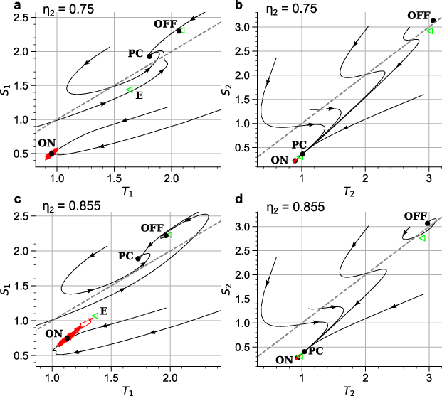
- Bifurcation diagram: A plot showing the equilibria or dynamics of a system as a parameter varies, highlighting qualitative changes. "Bifurcation diagrams of the box model with respect to the freshwater forcing parameter η2"
- Bifurcation-induced tipping point (TP): An abrupt transition caused by a bifurcation where stability is lost. "This is a bifurcation-induced tipping point (TP)"
- Bistability: The coexistence of two stable states under the same external conditions. "a bistability of the AMOC was shown in a conceptual model"
- Box model: A simplified compartmental model representing parts of the ocean with averaged properties. "A Stommel-type box model is presented"
- Center manifold theorem: A mathematical result ensuring that dynamics near a bifurcation can be reduced to a lower-dimensional manifold. "For saddle-node bifurcations in higher-dimensional systems the picture of Fig.~\ref{fig:csd} applies locally in phase space when close to the bifurcation due to the center manifold theorem."
- Critical slowing down (CSD): The slowing of a system’s recovery rate near a loss of stability, causing increased variance and autocorrelation. "These arise due to critical slowing down (CSD) before bifurcations"
- Downwelling: The sinking of surface water to deeper layers in the ocean. "the AMOC's current downwelling path"
- Early-warning signals (EWS): Statistical indicators, such as rising variance or autocorrelation, that precede tipping. "An alternative are early-warning signals (EWS) in AMOC fingerprints"
- Eddy-resolving model: A high-resolution ocean model that explicitly simulates mesoscale eddies. "an eddy-resolving ocean-only model recently simulated an AMOC collapse"
- Edge state: An unstable state on the boundary between basins of attraction that governs transitions. "also known as the edge state"
- Ensemble simulations: Multiple runs of a model with different initial conditions or stochastic realizations to quantify uncertainty. "ensemble simulations with a single model where some ensemble members in intermediate scenarios reach a weak AMOC state and other do not"
- Euler–Maruyama scheme: A numerical method for integrating stochastic differential equations. "simulations are performed with an Euler-Maruyama scheme"
- Fingerprint (climate): A characteristic spatial or temporal pattern used as a proxy for a system’s state or forcing. "A 'fingerprint' based on subpolar gyre temperatures is shown"
- Fold bifurcation: A bifurcation (saddle-node) where a stable and an unstable fixed point collide and annihilate. "fold bifurcations of two saddle points"
- Freshwater forcing: Input of freshwater (e.g., from ice melt or precipitation) that alters ocean salinity and density. "the freshwater forcing needed for an AMOC shutdown are quite high and model dependent"
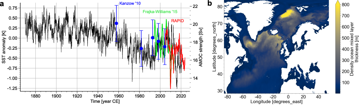
- Hydrographic sections: Oceanographic transects measuring temperature, salinity, and other properties across specified lines. "Five hydrographic sections in the period 1957-2004"
- Internal variability: Natural variability intrinsic to the climate system without changes in external forcing. "Model averages remove internal variability"
- Lag-1 autocorrelation: Autocorrelation at a one-step time lag, often used to detect memory increase near tipping. "For this process the lag-1 autocorrelation is given by ρ1 = e{- λ Δ t}"
- Linear equation of state: A linear relation expressing density as a function of temperature and salinity deviations from a reference. "the latter equality follows from a linear equation of state"
- Meridional density gradient: The north–south (meridional) difference in density that drives overturning circulation. "q_{1,2} ∝ ρ_{p1,2} - ρ_e" and "depends on the meridional density gradient between the equatorial and each of the polar boxes"
- Multistability: The coexistence of more than two stable states in a system. "To get any multistability with coexisting ON and OFF states, η3 needs to be sufficiently small"
- Noise-induced transitions: Jumps between stable states caused by random perturbations rather than parameter changes. "When close to the bifurcations, there are rare noise-induced transitions"
- Observable (dynamical systems): A measurable quantity, often a function of system variables, used to monitor state and fluctuations. "The term observable is used here either loosely as any quantity that can be measured"
- Operator-theoretic arguments: Analytical methods using linear operators (e.g., Koopman or transfer operators) to study dynamics and observables. "operator-theoretic arguments \cite{LUC24,LOH25b}"
- Ornstein–Uhlenbeck process: A mean-reverting Gaussian stochastic process used to approximate linearized dynamics with noise. "approximated by the Ornstein-Uhlenbeck process"
- OSNAP array: An observing system in the subpolar North Atlantic measuring overturning and transports. "and the OSNAP array (55-60°N, since 2014)"
- Petawatt (PW): A unit of power equal to 1015 watts, used to quantify ocean heat transport. "carrying 1.2 PW of heat northward across the subtropics"
- Phase portrait: A plot of trajectories or flow in state space illustrating system dynamics. "Projected phase portraits of the AMOC box model"
- Polar amplification: Stronger warming at high latitudes compared to the global average. "due to polar amplification of global warming"
- Quasi-steady state simulations: Long integrations approximating equilibrium responses to forcing. "Full collapses were identified in quasi-steady state simulations with different models"
- Quasipotential: A potential-like function describing stability and transition pathways in stochastic systems. "or more generally quasipotential"
- RAPID–MOCHA array: A mooring array at ~26.5°N for continuous AMOC monitoring. "The RAPID-MOCHA array (at 26.5°N, since 2004)"
- Restoring rate (λ): The linear rate at which perturbations decay back to a stable state. "with a restoring rate λ going to zero"
- Saddle-node bifurcation: A bifurcation where a stable node and a saddle coalesce and disappear, causing loss of stability. "a saddle-node bifurcation can occur"
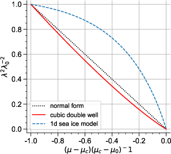
- Saddle-node normal form: The canonical one-dimensional equation describing dynamics near a saddle-node bifurcation. "the required scaling of variance or autocorrelation only arises when the observable obeys the saddle-node normal form"
- Salt-advection feedback: A positive feedback where circulation changes alter salinity advection, reinforcing weakening or strengthening. "Due the likely existence of the salt-advection feedback"
- Sea level anomalies: Deviations of sea level from a baseline, used as proxies for circulation changes. "Exploiting the correlation of RAPID AMOC strength and sea level anomalies"
- Sea surface temperature fingerprint: An SST-based pattern used as a proxy for AMOC strength. "The longest time series (black) is the sea surface temperature fingerprint"
- Spiciness (oceanographic): A temperature–salinity combination orthogonal to density, often represented as T+S. "aligned with Atlantic 'spiciness', i.e., T+S"
- Stochastic differential equation: A differential equation including a random (noise) term to model stochastic dynamics. "the state is then governed by the stochastic differential equation"
- Stommel-Cessi model: A conceptual AMOC model variant featuring quadratic dependence on density gradients. "data from the Stommel-Cessi model \cite{CES94} would give a too early prediction"
- Stommel’s model: The classic two-box model demonstrating AMOC bistability via temperature–salinity feedbacks. "As in Stommel's model \cite{STO61}, a reversed and weaker salinity-driven circulation state can exist"
- Subpolar gyre: A large-scale cyclonic circulation in the subpolar North Atlantic. "Shown is the anomaly of sea surface temperatures in the North Atlantic subpolar gyre"
- Sverdrup (Sv): A unit of volume transport equal to 106 m3 s-1, used for ocean circulation strength. "an AMOC weakening of about about 1 Sv in the period 1993-2014 was estimated"
- Tipping element: A subsystem of the Earth system susceptible to abrupt, nonlinear transitions. "which may be considered a separate tipping element"
- Tipping point (TP): A threshold at which a qualitative change in system state occurs. "the AMOC is indeed approaching a TP"
- Welander’s convective feedback: A positive feedback mechanism involving ocean convection proposed by Welander. "such as Welander's convective feedback"
- Wiener process: A mathematical model of Brownian motion used as the noise term in SDEs. "with a standard Wiener process W_{T_1,t}"
Collections
Sign up for free to add this paper to one or more collections.