Transient learning dynamics drive escape from sharp valleys in Stochastic Gradient Descent
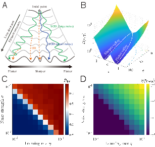
Abstract: Stochastic gradient descent (SGD) is central to deep learning, yet the dynamical origin of its preference for flatter, more generalizable solutions remains unclear. Here, by analyzing SGD learning dynamics, we identify a nonequilibrium mechanism governing solution selection. Numerical experiments reveal a transient exploratory phase in which SGD trajectories repeatedly escape sharp valleys and transition toward flatter regions of the loss landscape. By using a tractable physical model, we show that the SGD noise reshapes the landscape into an effective potential that favors flat solutions. Crucially, we uncover a transient freezing mechanism: as training proceeds, growing energy barriers suppress inter-valley transitions and ultimately trap the dynamics within a single basin. Increasing the SGD noise strength delays this freezing, which enhances convergence to flatter minima. Together, these results provide a unified physical framework linking learning dynamics, loss-landscape geometry, and generalization, and suggest principles for the design of more effective optimization algorithms.
Paper Prompts
Sign up for free to create and run prompts on this paper using GPT-5.
Top Community Prompts
Explain it Like I'm 14
Explaining “Transient Learning Dynamics Drive Escape from Sharp Valleys in Stochastic Gradient Descent”
1) Big Picture: What is this paper about?
This paper tries to answer a simple but important question in deep learning: Why does the most popular training method, called Stochastic Gradient Descent (SGD), so often find solutions that work well on new, unseen data? The authors’ main idea is that, early in training, the algorithm explores the “landscape” of possible settings in a special way that helps it escape bad spots (sharp valleys) and settle in better ones (flat valleys). They show that this early exploration is temporary, and eventually the system “freezes” into one valley—ideally a flatter one that generalizes better.
Think of training like hiking through a mountain range:
- The “loss landscape” is the terrain (lower is better).
- “Sharp valleys” are narrow, steep dips—easy to get stuck in but not reliable.
- “Flat valleys” are wide, gentle dips—harder to find but more stable and better for generalization.
- The “noise” in SGD acts like gusts of wind that help you try different paths and jump between valleys early on.
2) What questions are the authors asking?
- During the first part of training, how does SGD move through the loss landscape?
- Why does SGD tend to end up in flatter valleys that generalize better?
- How does the amount of randomness (noise) in SGD—controlled by the learning rate and batch size—affect where training ends up?
- Is there a simple physical explanation for this behavior?
3) How did they study it?
The authors combined experiments on real neural networks with a simple, physics-inspired model:
- Real training runs:
- They trained a small neural network on part of the MNIST handwriting dataset.
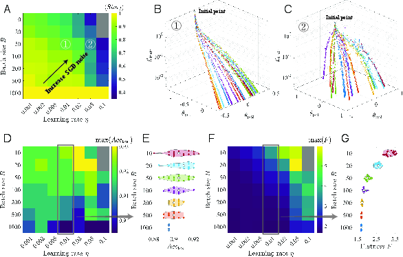
- They changed the learning rate and batch size to adjust the “noise” in SGD (bigger learning rate or smaller batch size = more noise).
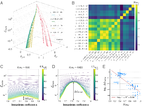
- They tracked where different runs ended up in the loss landscape and measured how “similar” the final models were by comparing which test images they got wrong (this avoids tricky issues like neuron order).
- They also measured how “flat” each solution was using the Hessian (a tool that, simply put, tells you how steep the landscape is in different directions).
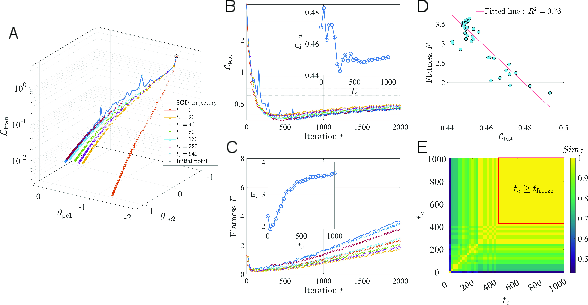
- Continuation training (an everyday analogy):
- Imagine you’re hiking with gusty wind (SGD) and occasionally pausing to walk with no wind (full-batch gradient descent, or GD).
- At different times, they “paused” the windy walk and switched to no wind to see which valley the model was currently in. This revealed when and how the model was hopping between valleys early in training.
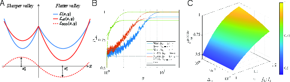
- A toy “two-valley” model:
- They built a simple math model with just two valleys: one sharp and one flat.
- They added landscape-aware noise (stronger in steeper directions) to mimic SGD’s randomness.
- This let them run many simulations and use known physics ideas to explain the behavior in plain terms.
4) What did they find, and why does it matter?
Here are the key results and their importance:
- Early training is an exploratory phase with “valley jumping”:
- At the start, SGD often moves between different valleys. It doesn’t get stuck right away.
- This is when it can escape sharp valleys and drift toward flatter ones.
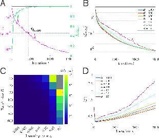
- The system “freezes” later:
- As training goes on, the landscape effectively grows barriers between valleys.
- Eventually, it becomes very hard to switch valleys—training “freezes” into one basin (valley).
- More noise = longer exploration = better valleys:
- Increasing noise (larger learning rate or smaller batch size) gives more time before freezing.
- With more time, the model is more likely to reach flatter valleys.
- Flatter valleys correlated strongly with better test performance, meaning better generalization.
- The noise reshapes the landscape in a helpful way:
- The randomness in SGD is not equal in all directions; it’s stronger where the landscape is steeper.
- This “anisotropic” noise effectively makes flat valleys more attractive and sharp valleys less attractive during the early phase.
- In the simple two-valley model, this shows up as an “effective potential” that favors flat regions.
- Continuation training directly shows the jumps:
- When switching from SGD (with noise) to GD (no noise) at different times, the final valley changes early on but stops changing after the freezing time. This is clear evidence of early valley-hopping.
Why it matters: It explains why SGD tends to find solutions that generalize well—not because sharp valleys are unstable or “forbidden,” but because early noise-driven exploration nudges the process toward flatter valleys before it freezes.
5) What are the implications?
- Early training matters a lot:
- The first part of training largely decides where you’ll end up. Managing that phase can improve results.
- Practical training tips:
- Using more noise early (for example, a larger learning rate or smaller batch size) can help the model explore and find flatter, better-generalizing solutions.
- Later, you can reduce noise to stabilize and fine-tune the solution.
- Better optimizer design:
- New algorithms might deliberately control noise and its direction to guide exploration.
- For instance, methods that keep noise longer in the early phase could improve generalization.
- Unifying view:
- The paper provides a physical, intuitive framework that links three things: the randomness in training, the shape of the loss landscape, and why models generalize.
In short, the paper shows that the “gusts of wind” in SGD early on are not just random—they’re exactly what helps the model escape narrow valleys and settle into wide, reliable ones. By understanding and controlling this early, transient exploration, we can train models that perform better in the real world.
Knowledge Gaps
Knowledge gaps, limitations, and open questions
Below is a concise, actionable list of what remains missing, uncertain, or unexplored in the paper, organized to guide future research:
- Empirical scope and scalability:
- Validate the transient “valley-jumping” and freezing phenomena on large-scale models (e.g., Transformers), datasets (e.g., ImageNet), and training regimes typical of modern practice.
- Test whether the reported trends hold under realistic training schedules (warmup, cosine decay, restarts, cyclical learning rates) where noise levels evolve non-monotonically.
- Assess robustness across explicit regularizers and components (weight decay, dropout, label smoothing, data augmentation, batch normalization, gradient clipping), which alter the noise structure and loss geometry.
- Optimizer dependence:
- Extend analyses beyond vanilla SGD to momentum SGD, Adam/AdamW, RMSProp, and SAM; quantify how adaptive preconditioning and momentum modify the effective noise, freezing time, and flat-minima bias.
- Determine whether the freezing mechanism competes with, complements, or overrides sharpness-aware procedures (e.g., SAM) and second-order methods.
- Noise characterization:
- Measure the gradient-noise covariance during training to empirically test the assumption Σ ∝ H (or more generally, its monotonic relation to H) and quantify anisotropy and landscape dependence in real networks.
- Account for non-Gaussian and heavy-tailed gradient noise observed in practice, and evaluate whether the freezing mechanism and effective potential persist under such noise.
- Disentangle contributions to stochasticity from mini-batch sampling versus other sources (dropout, data augmentation randomness, label noise).
- Theoretical assumptions and approximations:
- Clarify the stochastic calculus (Itô vs. Stratonovich) used for multiplicative, state-dependent noise; derive and test the implied noise-induced drift terms in the Fokker–Planck description.
- Quantify when the discrete-time SGD dynamics are well-approximated by the continuous-time Langevin limit; characterize deviations at practical learning rates where discretization artifacts are significant.
- Test the timescale separation (τx ≪ τy) in high-dimensional networks and identify conditions under which the quasi–steady-state approximation fails.
- Generalize the 2D two-valley model to multi-valley, high-dimensional settings with realistic topology (multiple bifurcations, saddles, curved valley networks), and examine whether predictions (e.g., scaling of freezing time with noise) remain valid.
- Relax toy-model constraints (equal valley depths, fixed flatness ratio with training progress, specific forms of L0(y)) and assess sensitivity of the theory to these choices.
- Quantitative validation of predictions:
- Rigorously test the predicted scaling of freezing time and flat-valley selection probability with effective noise ΔS = ησ and flatness contrast γ across different architectures/datasets.
- Empirically estimate barrier height growth and validate the derived formulae for y_freeze and P_flattr against measured inter-valley transition rates and barrier statistics in real training.
- Compare steady-state vs. transient-theory predictions quantitatively using measured noise and Hessian statistics, not only qualitatively.
- Measurement choices and flatness metrics:
- Evaluate alternative, scale-invariant flatness measures that are robust to reparameterization and normalization (e.g., filter-wise rescaling, batch-norm invariances), and compare with the chosen geometric mean of top Hessian eigenvalues.
- Probe how the choice of N (number of eigenvalues used) and spectrum tails affect the flatness–generalization link and conclusions.
- Complement linear interpolation with minimal-energy paths or geodesic mode connectivity to avoid overestimating barriers along straight lines.
- Identifying and tracking valleys:
- Develop more principled methods to label and track valleys during training (beyond PCA projection and Jaccard similarity of misclassifications) that are robust to symmetries and functionally equivalent parameterizations.
- Assess sensitivity of the valley identification to test-set size, class imbalance, and metric choice (e.g., calibration error, margin distributions), not just test accuracy or misclassification overlap.
- Continuation (switch-to-GD) protocol:
- Analyze how the specific continuation settings (learning rate, discretization, optimizer choice) affect which valley GD converges to; verify that continuation reliably reveals the valley occupied at branching time.
- Explore alternative deterministic projections (e.g., line search, very small LR, second-order steps) to reduce confounds from discretization and unstable directions when switching.
- Early-phase dynamics and initialization:
- Separate the effects of initialization randomness from SGD noise in determining early valley selection; quantify their relative contributions across seeds and data orders.
- Study how dataset size, class balance, and curriculum or data ordering influence barrier formation, freezing time, and valley-jumping dynamics.
- Beyond in-distribution accuracy:
- Test whether noise-delayed freezing that favors flatter minima also improves calibration, robustness (adversarial and corruption), and out-of-distribution generalization.
- Examine trade-offs (if any) between flatter-valley selection and other desiderata (e.g., training speed, stability under distribution shift).
- Practical algorithm design:
- Derive and validate actionable noise schedules (via batch size or LR) that deliberately extend the exploratory phase without incurring divergence, including adaptive controllers based on online estimates of freezing onset.
- Investigate whether targeted noise anisotropy (e.g., curvature-aware noise injection or preconditioning) can systematically steer training toward flatter regions more efficiently than uniform noise scaling.
- Landscape geometry during training:
- Directly measure how barrier heights, Hessian spectra, and flatness evolve with training time in real models to substantiate the proposed “barrier growth” and “valley flattening” mechanisms.
- Determine whether saddle point structures and negative curvature directions mediate valley transitions and how these interact with anisotropic noise.
- Generalization theory linkage:
- Connect the transient-freezing mechanism to formal generalization bounds (e.g., PAC-Bayes, margin-based) under realistic invariances, and reconcile cases where sharp minima can generalize well due to parameterization or scale invariance.
These gaps collectively point to the need for broader empirical validation, richer noise and optimizer modeling, more robust measurement protocols, and quantitative tests of the theory’s predictions in high-dimensional, large-scale training regimes.
Practical Applications
Below are practical applications drawn from the paper’s findings on transient learning dynamics, SGD noise, and valley selection. Each item notes sector relevance, potential tools or workflows, and key assumptions or dependencies that affect feasibility.
Immediate Applications
- Adaptive noise scheduling to improve generalization in deep learning
- Sectors: software/ML across industry (recommendation, search, ads), healthcare (diagnostics), finance (risk modeling), robotics (perception)
- Workflow: start training with higher SGD noise (smaller batch sizes and/or larger learning rates) to delay freezing and encourage valley jumping, then anneal noise (increase batch size or reduce learning rate) once training loss crosses a low threshold (e.g., L_c≈0.1)
- Tools/products: “NoiseScheduler” plugin for PyTorch/TF that maintains a target effective noise Δ_S early and reduces it post-freezing
- Assumptions/dependencies: flatness–generalization link holds; stability constraints (avoid divergence at high LR); datasets and architectures similar enough for early-phase dynamics to matter
- Freezing-time monitoring to time hyperparameter transitions and checkpoint selection
- Sectors: software/ML MLOps, healthcare model governance, finance model risk management
- Workflow: monitor training loss to detect freezing time t_freeze; switch optimizer settings (e.g., LR, batch size, weight decay) or trigger checkpoint selection before or at freezing
- Tools/products: “FreezeWatch” module that signals t_freeze and automates schedule changes and checkpointing
- Assumptions/dependencies: choice of L_c threshold requires tuning; reliable training-loss measurement under stochasticity; minimal overhead
- Continuation training for valley identification and model selection
- Sectors: ML research and production, healthcare AI QA, high-stakes decision systems (credit scoring)
- Workflow: branch runs at early checkpoints to deterministic GD (large batch, same LR) to reveal which valley the trajectory occupies; select branches that land in flatter, lower test-loss minima
- Tools/products: “ValleyScout” workflow integrated into training pipelines to periodically branch and score valleys
- Assumptions/dependencies: extra compute budget; deterministic GD converges within the local basin; valley quality correlates with generalization on target data
- Flatness tracking during training as a proxy for generalization
- Sectors: ML model development across industries; education (ML courses/labs)
- Workflow: estimate top Hessian eigenvalues or proxies (e.g., sharpness measures, trace via Hutchinson/Lanczos) at checkpoints to track increasing flatness; use as early stopping or selection criterion
- Tools/products: “FlatnessTracker” library providing scalable Hessian proxies and alerts when flatness plateaus or declines
- Assumptions/dependencies: computational feasibility for large models; flatness proxy fidelity; correlation between flatness metrics and test performance for the specific task
- Diversity-aware training and selection via controlled noise
- Sectors: recommendation systems, ensemble methods in healthcare/finance, AutoML
- Workflow: run multiple seeds with elevated early noise to explore diverse valleys; select or ensemble flatter solutions (e.g., stochastic weight averaging across valley floors)
- Tools/products: pipeline template for “ValleyDiversity” runs, with automated ranking by flatness and test loss; optional SWA integration
- Assumptions/dependencies: additional training runs are affordable; ensembling complements the application’s latency/size constraints
- Curriculum-level regularization aligned with transient exploration
- Sectors: computer vision (data augmentation), NLP (masking), robotics (domain randomization)
- Workflow: amplify early-stage regularization (augmentation intensity, dropout, label smoothing) to mimic/boost effective exploration; taper regularization post-freezing
- Tools/products: curriculum schedulers that co-tune augmentation intensity with batch size/LR
- Assumptions/dependencies: regularization interacts constructively with SGD noise; task-specific tuning required to avoid underfitting
- Diagnostics for premature freezing (early overfitting risk)
- Sectors: production ML QA, safety-critical ML (medical, autonomous systems)
- Workflow: detect too-early freezing (small t_freeze) and respond by increasing early noise (reduce batch size, increase LR), or intensify augmentation
- Tools/products: training dashboards with “Freeze Health” indicators; automated corrective actions
- Assumptions/dependencies: reliable detection under noisy loss traces; guardrails to avoid instability when increasing noise
Long-Term Applications
- Transient-aware optimizers that actively control freezing dynamics
- Sectors: ML platforms, foundation model training, robotics RL
- Workflow: design optimizers that estimate escape rates/barrier heights and adapt LR/noise to keep τ_escape comparable to τ_y until desired exploration is achieved, then intentionally “freeze” into selected basins
- Tools/products: “AnisoSGD” or “FreezeControl” optimizers using Hessian approximations (KFAC, diagonal Fisher) to shape anisotropic noise
- Assumptions/dependencies: scalable curvature estimation; robust control laws to prevent instability; validation across architectures and data regimes
- Hessian-aligned noise injection and landscape engineering
- Sectors: advanced optimization research, AutoML, scientific ML
- Workflow: inject anisotropic noise proportional to estimated Hessian or its powers to reproduce the effective potential that favors flat valleys; or add explicit loss corrections approximating the SGD-induced effective potential
- Tools/products: curvature-aware noise modules; “EffectiveLoss” regularizers mimicking the SGD correction term
- Assumptions/dependencies: practical, low-cost Hessian estimation; theoretical guarantees for convergence and generalization; interplay with existing regularizers (weight decay, batch norm)
- Valley mapping and landscape analytics platforms
- Sectors: MLOps, academia, regulatory auditing
- Workflow: routinely map valleys via continuation branches, interpolation barriers, and error-set similarity (Jaccard of misclassifications); archive valley metadata for model selection and audits
- Tools/products: “ValleyLens” service offering barrier profiles, similarity matrices, and flatness summaries per run
- Assumptions/dependencies: storage/compute overhead; standardized metrics across tasks; benefits justify operational complexity
- Meta-learning of noise schedules and freezing-time policies
- Sectors: AutoML, foundation model training at scale
- Workflow: learn task-specific schedules for LR, batch size, augmentation intensity to maximize final flatness and test performance, conditioned on early loss/flatness signals
- Tools/products: schedule controllers trained via Bayesian optimization/RL; schema for exporting learned policies across tasks
- Assumptions/dependencies: reliable early predictors of valley quality; transferability of learned schedules; guardrails against overfitting schedules to specific datasets
- Federated and distributed training strategies that promote global generalization
- Sectors: mobile/edge AI, healthcare consortia, finance consortia
- Workflow: coordinate client-side early high-noise phases to reach flatter minima that generalize across heterogeneous data, followed by synchronized freezing/aggregation
- Tools/products: federated “Noise-Orchestrator” controlling client batch/LR; valley-consensus protocols using flatness and error similarity
- Assumptions/dependencies: communication constraints; heterogeneous hardware; privacy limits on curvature estimates
- Robustness and reliability certification via flatness and barrier metrics
- Sectors: safety-critical ML (medical devices, autonomous driving), policy/regulation
- Workflow: integrate flatness measures, barrier heights, and valley diversity into model documentation and certification as indicators of generalization and stability
- Tools/products: “Generalization Card” standards with prescribed metrics; auditing tools
- Assumptions/dependencies: community consensus that flatness proxies reflect robustness; standardized, reproducible computation of metrics
- Hardware–software co-design for phase-aware training
- Sectors: AI accelerators, cloud providers
- Workflow: optimize early training for small batches/high noise (memory bandwidth, kernel scheduling), then switch to large-batch efficiency post-freezing
- Tools/products: runtime schedulers that reconfigure kernels and memory plans across phases; cost-aware training policies
- Assumptions/dependencies: hardware support for dynamic batch/LR changes; measurable ROI in time-to-accuracy and generalization
- Extensions to reinforcement learning and continual learning
- Sectors: robotics, autonomous systems, adaptive user modeling
- Workflow: adapt exploration–exploitation schedules using freezing analogs (maintain higher exploration until policy reaches flatter basins), and in continual learning add noise to avoid premature freezing in previous-task basins
- Tools/products: RL “Freeze-Aware” explorers; continual-learning noise controllers
- Assumptions/dependencies: mapping SGD valley dynamics to RL optimization; task-specific stability and performance validation
- Education and training materials on transient learning dynamics
- Sectors: academia, professional training
- Workflow: curriculum modules and lab exercises demonstrating valley jumping, freezing time detection, continuation training, and noise scheduling
- Tools/products: teaching notebooks, interactive visualizations of loss landscapes and trajectories
- Assumptions/dependencies: simplified models that illustrate phenomena without excessive compute; alignment with program outcomes
Across these applications, core dependencies include: the empirical flatness–generalization relationship; the feasibility of estimating curvature (Hessian) at scale; careful tuning to avoid divergence under high early noise; compute overhead for continuation and analytics; and validation across architectures (CNNs, transformers) and datasets.
Glossary
- Activity–weight duality: A theoretical relation showing an explicit link between solution flatness and generalization in deep networks. Example: "an exact activity-weight duality"
- Anisotropic diffusion tensor: A direction-dependent diffusion matrix governing stochastic dynamics, reflecting unequal variance across directions. Example: "an anisotropic diffusion tensor"
- Anisotropic noise: Noise whose magnitude varies by direction, often aligned with curvature of the loss landscape. Example: "Anisotropic noise in SGD reshapes the loss landscape"
- Basin of attraction: The region of parameter space whose points flow to the same local minimum under the optimizer’s dynamics. Example: "confined to the basin of attraction of a single valley"
- Bifurcating valley: A valley in the loss landscape that splits into two branches as a control direction changes. Example: "takes the form of a bifurcating valley"
- Bifurcation scale: The parameter setting the point or rate at which a valley splits into branches. Example: "sets the bifurcation scale"
- Continuation training: A procedure that switches from SGD to deterministic GD at a chosen time to identify the valley currently occupied. Example: "a {\it continuation training} experiment"
- Drift term: A deterministic component added to the loss to model global downward bias during training. Example: "we introduce a global drift term"
- Effective noise level: The product of learning rate and noise strength that determines overall stochasticity in continuous approximations of SGD. Example: "the effective noise level of SGD is defined as"
- Effective potential: A noise-induced landscape that the dynamics effectively experience, biasing trajectories (e.g., toward flatter minima). Example: "an effective potential that favors flat solutions"
- Effective temperature: A scalar that rescales the steady-state distribution, analogous to temperature in statistical physics. Example: "denotes the effective temperature"
- Energy barriers: Obstacles between valleys that increase the time required to transition from one minimum to another. Example: "growing energy barriers suppress inter-valley transitions"
- Equilibrium steady state (ESS): The stationary distribution expected under equilibrium conditions satisfying detailed balance. Example: "The equilibrium steady-state (ESS) probability"
- Fokker–Planck equation: A partial differential equation describing the time evolution of a probability density under drift and diffusion. Example: "according to a corresponding Fokker--Planck equation"
- Freezing time: The moment when training enters a low-loss regime and exploration effectively ceases. Example: "freezing time"
- Fluctuation–dissipation theorem: A principle relating noise (fluctuations) to dissipation; its violation indicates nonequilibrium dynamics. Example: "violates the fluctuation–dissipation theorem"
- Flatness: A measure of how wide or gently curved a minimum is, often linked to better generalization. Example: "flatness is quantified as"
- Flatness ratio: The relative flatness between two valleys, often denoted γ, comparing their inverse curvatures. Example: "We define this flatness ratio as"
- Geometric mean: The multiplicative average used here to aggregate top Hessian eigenvalues when defining flatness. Example: "inverse geometric mean of the top N non-degenerate Hessian eigenvalues"
- Hessian: The matrix of second derivatives of the loss with respect to parameters, capturing local curvature. Example: "aligns with the Hessian matrix"
- Hessian eigenvalues: The eigenvalues of the Hessian that quantify curvature along principal directions. Example: "top N non-degenerate Hessian eigenvalues"
- Hessian spectrum: The full set (distribution) of Hessian eigenvalues used to characterize curvature structure. Example: "Hessian spectra computed at these endpoints provide additional evidence"
- Imaginary error function (erfi): A special function used in rate expressions for escape over barriers. Example: "denotes the imaginary error function"
- Inter-valley transitions: Stochastic moves between distinct minima separated by barriers. Example: "suppress inter-valley transitions"
- Jaccard similarity: A set-overlap metric (intersection over union) used here to compare misclassification sets between solutions. Example: "Pairwise Jaccard similarity"
- Kramers’ rate theory: A theory estimating escape rates over energy barriers under stochastic dynamics. Example: "we apply Kramers’ rate theory to estimate the escape rates"
- Langevin equation: A stochastic differential (or difference) equation describing gradient flow with noise. Example: "a discrete-time Langevin equation"
- Landscape-dependent noise: Gradient noise whose covariance depends on local curvature (e.g., proportional to the Hessian). Example: "To capture this landscape-dependent noise"
- Linear interpolation path: A straight-line path in parameter space between two solutions used to probe barriers. Example: "the linear interpolation path"
- Loss barrier: The increase in loss encountered along a path between two minima, quantifying separation between valleys. Example: "define the loss barrier"
- Loss landscape: The function mapping parameters to loss, viewed as a high-dimensional surface with valleys and barriers. Example: "the geometry of this loss landscape"
- Nonequilibrium mechanism: A process operating without detailed balance that biases learning dynamics (e.g., due to anisotropic noise). Example: "identify a nonequilibrium mechanism"
- Nonequilibrium steady state (NESS): A stationary distribution under persistent probability currents or anisotropic noise, not satisfying equilibrium constraints. Example: "nonequilibrium steady-state (NESS) predictions"
- Principal Component Analysis (PCA): A dimensionality-reduction method used to visualize high-dimensional training trajectories. Example: "Principal Component Analysis (PCA) projection"
- Permutation symmetry (of neurons): The invariance of network function under reordering of neurons, complicating direct weight-space comparisons. Example: "permutation symmetry of neurons"
- Quasi–steady-state: A regime where fast variables equilibrate conditionally while slow variables evolve. Example: "quasi-steady-state regime"
- Valley-jumping: The stochastic hopping between distinct valleys during early training. Example: "valley-jumping"
- Waddington epigenetic landscape: A metaphorical landscape from developmental biology used to illustrate bifurcating paths to stable fates. Example: "the Waddington epigenetic landscape"
Collections
Sign up for free to add this paper to one or more collections.