Manifold constrained steepest descent
Abstract: Norm-constrained linear minimization oracle (LMO)-based optimizers such as spectral gradient descent and Muon are attractive in large-scale learning, but extending them to manifold-constrained problems is nontrivial and often leads to nested-loop schemes that solve tangent-space subproblems iteratively. We propose \emph{Manifold Constrained Steepest Descent} (MCSD), a single-loop framework for optimization over manifolds that selects a norm-induced steepest-descent direction via an LMO applied to the Riemannian gradient, and then returns to the manifold via projection. Under standard smoothness assumptions, we establish convergence guarantees for MCSD and a stochastic momentum variant. We further introduce \emph{SPEL}, the spectral-norm specialization of MCSD on the Stiefel manifold, which admits scalable implementations via fast matrix sign computations. Experiments on PCA, orthogonality-constrained CNNs, and manifold-constrained LLM adapter tuning demonstrate improved stability and competitive performance relative to standard Riemannian baselines and existing manifold-aware LMO methods.

Paper Prompts
Sign up for free to create and run prompts on this paper using GPT-5.
Top Community Prompts
Explain it Like I'm 14
Overview
This paper introduces a new way to train machine learning models when their parameters must stay on a special curved surface (called a “manifold”). The method is called Manifold Constrained Steepest Descent (MCSD). It helps you move “downhill” to reduce loss while staying on the manifold, using a simple update step that is fast and has mathematical guarantees that it will make progress. The authors also present a practical version for a common manifold used in deep learning (the Stiefel manifold), called SPEL, and show it works well on tasks like PCA, training CNNs with orthogonal weights, and fine-tuning LLMs.
Key Objectives and Questions
The paper asks straightforward questions:
- Can we create a simple, single-loop optimizer for manifold-constrained problems that is as easy to run as popular Euclidean methods (like gradient descent), but still respects the manifold?
- Can we pick “steepest descent” directions using a tool called a linear minimization oracle (LMO) under different norms, and then project back to the manifold in one step?
- Can we prove that this optimizer actually converges (makes steady progress) in both standard and noisy (stochastic) training?
- Can we build a practical version for the Stiefel manifold (orthogonality constraints), and does it work well on real tasks?
Methods and Approach (with simple analogies)
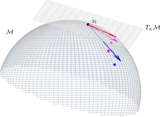
Think of training as walking downhill on a landscape to reach a valley (the best solution). On flat ground (ordinary Euclidean space), you can step directly downhill. On a curved surface (a manifold), like a sphere or a surface of “orthogonal matrices,” stepping straight downhill often takes you off the surface. You must:
- choose a smart downhill direction on the surface, and
- get back onto the surface after moving.
Here’s what the paper does:
- Riemannian gradient: This is like the “on-surface” version of the usual gradient. It tells you the best local downhill direction that keeps you aligned with the manifold’s geometry.
- LMO (Linear Minimization Oracle): This is a tool that, given a “slope” (like the gradient), picks a unit step direction that most reduces the loss under a chosen norm (think of a norm as a ruler that measures step sizes). Different norms give different kinds of “steepest” directions.
- MCSD update (single loop): Each iteration does two simple things: 1) Use the LMO on the Riemannian gradient to pick a steepest descent direction under your chosen norm. 2) Take a step, then project back to the manifold (like snapping back to the surface) using a fast projection.
Why is this useful? Many earlier manifold-aware LMO methods needed a slow “inner loop” to solve a hard subproblem in the tangent space (the surface’s local flat approximation). MCSD avoids that: it uses a direct LMO and a projection, so there’s just one loop.
Stiefel manifold and SPEL:
- The Stiefel manifold is the set of all matrices whose columns are orthonormal (like perfectly perpendicular, unit-length vectors). This shows up when you want weights to be orthogonal (helpful for stability and generalization).
- SPEL is MCSD specialized to the Stiefel manifold with the spectral norm (a matrix norm linked to its largest singular value). It uses:
- a simple LMO direction based on the spectral norm,
- a fast “matrix sign” projection that snaps the updated matrix back to the closest orthogonal one.
- These operations are efficient on GPUs, so SPEL is practical at scale.
The paper also gives a stochastic variant (like adding momentum and using noisy gradients from mini-batches), similar to common deep learning optimizers.
Main Findings and Why They Matter
The authors prove convergence:
- Deterministic MCSD: Under standard smoothness conditions (the loss doesn’t change wildly), MCSD’s simple steps guarantee progress toward a stationary point (where the gradient is small).
- Stochastic MCSD (with momentum): Even with noisy gradients (like in deep learning), the method still converges at a standard rate for first-order methods.
They also show practical benefits in experiments:
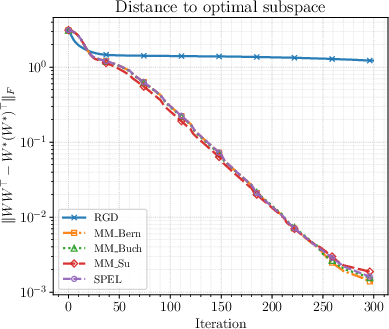
- PCA (a classic test): SPEL reaches similar accuracy to more complex manifold-LMO baselines but runs much faster, because it avoids nested inner loops.
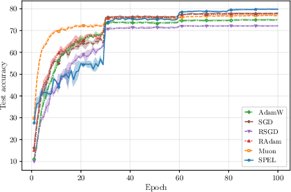
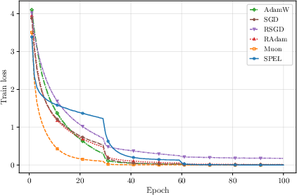
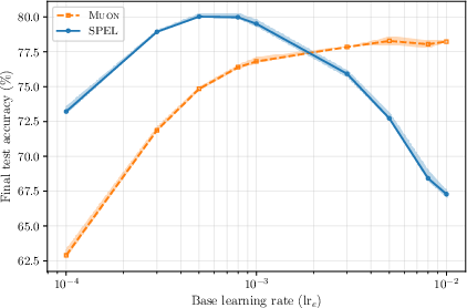
- Orthogonality-constrained CNNs on CIFAR-100: SPEL achieves the best final test accuracy among tested optimizers and remains stable across a wide range of learning rates.
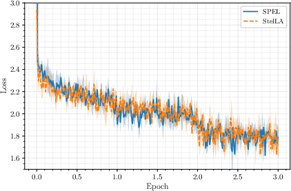
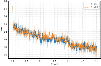
- LLM adapter tuning (StelLA adapters on LLaMA models): SPEL matches the accuracy of the existing manifold-aware optimizer while using lighter optimizer state, making it attractive for large-scale training.
These results matter because:
- They provide a simple, efficient, and theoretically sound way to optimize on manifolds.
- They show that orthogonality constraints (on CNNs, adapters, etc.) can be enforced reliably with competitive or superior performance.
- They bridge ideas from modern Euclidean optimizers (like spectral-LMO methods) to the manifold setting.
Implications and Potential Impact
This work offers a practical toolkit for training models with geometric constraints:
- Simpler and faster: MCSD’s single-loop design is easier to implement and tune than methods that require inner solvers.
- Scalable: SPEL uses GPU-friendly building blocks (like matrix sign), making it suitable for big models.
- Reliable: Convergence guarantees give users confidence the method will behave well.
- Broadly useful: Orthogonality and manifold constraints pop up in PCA, stable CNNs, robust training (Lipschitz control), and parameter-efficient LLM tuning. MCSD and SPEL make these applications more accessible and effective.
In short, the paper helps transform “optimization on curved surfaces” from something complicated and slow into something straightforward, fast, and well-supported by theory—useful for both classic algorithms and modern deep learning.
Knowledge Gaps
Knowledge gaps, limitations, and open questions
Below is a single, concrete list of what remains missing, uncertain, or unexplored in the paper, framed to guide future research:
- Scope beyond Stiefel: Despite presenting MCSD for general embedded manifolds, all algorithmic specializations, explicit constants, and experiments focus on the Stiefel manifold; applicability and efficiency on other manifolds (e.g., Grassmann, SPD, fixed-rank, Lie groups, hyperbolic) are not demonstrated or analyzed.
- Projection availability and uniqueness: MCSD assumes that the Euclidean projection P_M exists, is efficiently computable, and is single-valued in a neighborhood of the manifold; many manifolds lack a cheap or globally unique projection, and the paper does not characterize when MCSD is practically applicable (beyond Stiefel) or how non-uniqueness affects convergence.
- Inexact primitives: The theory assumes exact LMO and exact projection, whereas implementations use approximate matrix sign and numerical projections; robustness of MCSD/SPEL to inexact LMOs, approximate projections, or early-stopped iterations is not analyzed.
- Step-size selection in practice: Convergence requires staying within a tubular neighborhood (α_t ≤ r), but practical step-size rules (e.g., linesearch, adaptive schedules) that ensure feasibility and good progress without knowing r or L are not provided or analyzed.
- Conservative constants and neighborhood size: For Stiefel, the derived neighborhood (r = 0.2) and Lipschitz constant (L = 4L_f + 25G) may be highly conservative; how these bounds impact practical step sizes, and whether sharper constants can be obtained, is not investigated.
- Stationarity measure and rates: The guarantees are stated in terms of the dual norm of the Riemannian gradient and yield a T{-1/4} rate in the stochastic case—slower than common O(T{-1/2}) nonconvex SGD bounds; it is unclear if the analysis can be tightened or if stronger rates are obtainable for MCSD/SPEL.
- Comparison to tangent-space LMOs: MCSD chooses search directions in the ambient space (LMO on ∇_M f) instead of solving tangent LMO subproblems; formal comparisons (e.g., angle/alignment, sufficient-descent constants, local convergence behavior) with tangent-based methods (Manifold Muon variants) are not provided.
- Lack of curvature-aware or second-order variants: The framework selects steepest-descent directions under a norm but does not explore curvature-aware versions (e.g., trust-region, quasi-Newton, natural-gradient/metric-aware steps) or whether combining LMOs with second-order information improves performance.
- Momentum and transport: The stochastic variant uses heavy-ball momentum with simple tangent projection P_{T_xM}(m_t), bypassing vector transport/parallel transport; the impact of this approximation on bias, stability, and convergence, especially on curved manifolds, is not analyzed.
- Norm choices beyond spectral: Although the framework supports arbitrary norms, only the spectral norm is instantiated and evaluated; the trade-offs (theory/efficiency) for other norms (e.g., Frobenius, nuclear, group norms, block norms) on different manifolds remain unexplored.
- Interaction between projection and descent magnitude: Projection may substantially distort the effective step; there is no analysis of step-length contraction/expansion induced by P_M or of mechanisms to control it (e.g., projection-aware line-search).
- Constraints beyond smooth embedded manifolds: The approach is not analyzed for product manifolds with heterogeneous factors, quotient manifolds, or constraints with boundaries/non-smooth structure; consequences when P_M is only piecewise smooth or undefined are not discussed.
- Non-smooth objectives and regularization: The analysis assumes smooth f; extensions to composite objectives (e.g., smooth loss + nonsmooth regularizers), proximal variants, or projection-prox updates are not considered.
- Saddle-point behavior and second-order stationarity: Like many first-order methods, the analysis targets first-order stationarity; escaping strict saddles, second-order stationarity, or convergence to local minima is not studied.
- Large-scale implementation costs: SPEL relies on repeated matrix sign computations; the paper does not quantify end-to-end GPU/TPU throughput, memory bandwidth sensitivity, or scaling behavior for very large layers beyond the presented settings.
- Fairness and robustness of baselines: Manifold Muon baselines cap inner solves at 10 iterations with fixed configurations; how varying inner-solver accuracy affects the speed/accuracy trade-off and whether more optimized implementations change conclusions is left open.
- Coverage of tasks and manifolds in experiments: Experiments evaluate only PCA, orthogonality-constrained CNNs, and Stiefel-constrained LLM adapters; generalization to other tasks, architectures, or manifolds (e.g., fixed-rank factorization, spectral manifolds of SPD matrices) is not empirically validated.
- Hyperparameter transferability: While SPEL shows reasonable learning-rate sensitivity in the tested settings, there is no systematic study of hyperparameter transfer across architectures, datasets, and manifolds, or of layerwise scaling rules beyond those borrowed from Muon.
- Interaction with weight decay and regularization: The effect of weight decay/regularization in MCSD/SPEL under manifold constraints (and whether projection interferes with decoupled weight decay schemes) is not analyzed.
- Theoretical benefits vs. Riemannian GD: The work does not identify regimes where MCSD/SPEL provably outperform Riemannian GD (e.g., oracle complexity, dependence on condition numbers, or norm-induced geometry), leaving open when and why LMO-based manifold steps provide an advantage.
Practical Applications
Immediate Applications
Below are deployable applications that use the paper’s MCSD framework and its Stiefel specialization (SPEL) with existing projections and LMOs. Each item includes target sectors, possible tools/workflows, and feasibility notes.
- Orthogonality-constrained CNN training for stability and generalization (software/AI; healthcare imaging, autonomous driving, edge AI)
- What to do: Replace Riemannian optimizers or unconstrained training with SPEL on convolution kernels reshaped to Stiefel matrices; keep other parameters on standard optimizers (e.g., AdamW).
- Why it helps: Single-loop, projection-based updates enforce orthogonality throughout training, improving stability and often accuracy; per-iteration cost similar to RGD plus one matrix-sign (polar) computation.
- Tools/workflows: A PyTorch/JAX optimizer plugin “SPEL” that tags Stiefel parameters; uses GPU-friendly Polar Express or Newton–Schulz for msign; layerwise LR scaling as in Muon.
- Assumptions/dependencies: Efficient projection via msign available on GPU; tasks benefit from orthogonality (e.g., Lipschitz control, conditioning); standard smoothness for step-size stability.
- Parameter-efficient LLM adapter tuning with StelLA + SPEL (software/AI; finance/customer support/enterprise chat)
- What to do: Swap StelLA’s optimizer for SPEL on Stiefel-constrained adapter factors while keeping AdamW for unconstrained parameters.
- Why it helps: Matches StelLA’s accuracy with reduced optimizer state (no second-moment buffers for constrained blocks) and single-loop simplicity.
- Tools/workflows: Drop-in SPEL optimizer in existing adapter codebases; keep the same warm-up, decay, and layerwise LR scaling; runs on common GPUs (A100/H100).
- Assumptions/dependencies: Availability of StelLA/LoRA-style adapters; proper LR scaling; adequate GPU memory for msign; similar convergence conditions as in the paper.
- Faster PCA/subspace learning in data pipelines (finance risk, recommender systems, manufacturing analytics)
- What to do: Use MCSD/SPEL on Stiefel-constrained PCA (including Brockett cost) to accelerate convergence vs nested-loop manifold LMOs.
- Why it helps: Single-loop updates with polar projection reduce wall-clock time while preserving feasibility and convergence.
- Tools/workflows: Integrate into Spark/SQL ETL jobs or scikit-learn/skorch as a “StiefelPCA(SPEL)” estimator; GPU-accelerated polar operations for large n×p.
- Assumptions/dependencies: Data centered and objective smooth; efficient msign on target hardware; step-size schedules within the local projection radius.
- Online/streaming PCA with stochastic MCSD (IoT/edge analytics, anomaly detection)
- What to do: Apply the momentum-based stochastic MCSD for streaming subspace tracking under Stiefel constraints.
- Why it helps: Provable convergence under unbiased, bounded-variance gradients; maintains orthogonality without nested solves.
- Tools/workflows: Streaming operators that maintain a running covariance sketch and take SPEL updates per mini-batch.
- Assumptions/dependencies: Unbiased sub-sampled gradients or incremental estimates; variance control; stable step sizes.
- Attitude and pose optimization on SO(3) via MCSD + polar projection (robotics/aerospace)
- What to do: Optimize over rotation matrices with MCSD using projection Y→msign(Y) to enforce SO(3) constraints (or QR-based projection with det=+1 fix).
- Why it helps: Single-loop, fast small-matrix projections (3×3), robust to noise; useful in calibration, control, bundle adjustment substeps.
- Tools/workflows: Embedded control libraries adding “MCSD-Rotation” optimizer; differentiable projection for learning-based controllers.
- Assumptions/dependencies: Local smoothness of objective; small matrix sizes keep projection overhead negligible; care with det(+1) enforcement.
- Beamforming/precoder optimization with Stiefel constraints (telecom)
- What to do: Use SPEL to design orthonormal precoders/combiners under spectral-norm steepest descent.
- Why it helps: Maintains column orthogonality throughout iterations; avoids inner tangent-space solves.
- Tools/workflows: Integrate into MIMO design toolboxes; batch solve across channels; GPU execution for large antenna arrays.
- Assumptions/dependencies: Channel models yield smooth differentiable objectives; fast polar projections on matrices of practical sizes.
- Fixed-rank matrix factorization via MCSD + truncated SVD projection (recommender systems, system ID)
- What to do: Use MCSD with projection onto fixed-rank manifolds (via truncated SVD) for low-rank objectives.
- Why it helps: Single-loop updates leveraging efficient TSVD; no nested LMO inner solves.
- Tools/workflows: “MCSD-LowRank” module in recommender engines; TSVD via randomized SVD for speed.
- Assumptions/dependencies: Fast and accurate TSVD available; objective smoothness; memory fits intermediate factors.
- Robust/Lipschitz-controlled training using orthogonality constraints (healthcare diagnostics, safety-critical AI)
- What to do: Enforce orthogonality on selected layers to control Lipschitz constants; train with SPEL to maintain constraints exactly.
- Why it helps: Supports robustness-aimed pipelines (e.g., certified or empirical robustness) by keeping the spectral properties in check.
- Tools/workflows: Security/compliance training recipes that flag layers for Stiefel constraints; audit artifacts record constraint satisfaction per epoch.
- Assumptions/dependencies: System-level robustness depends on broader design (e.g., activation functions); orthogonality alone doesn’t guarantee certification.
- Optimizer-library extensions (software tooling)
- What to do: Provide MCSD/SPEL as drop-in optimizers in PyTorch/TF/JAX (torch.optim, Optax, etc.) with per-parameter geometry tags.
- Why it helps: Consistent, unified interface for manifold-constrained optimization with convergence guarantees; minimal changes to model code.
- Tools/workflows: “torch-optim-mcsd”, “optax-mcsd” with support for Stiefel, fixed-rank, and spectral manifolds; GPU kernels for msign.
- Assumptions/dependencies: Mature projection/LMO implementations; testing on common model archetypes; documentation for LR scaling and step-size ranges.
Long-Term Applications
These applications require further research, scaling work, or engineering before broad deployment.
- Foundation-model pretraining with manifold constraints at scale (software/AI)
- Vision: Enforce orthogonality/unitarity throughout Transformers using SPEL-like updates to improve stability and conditioning at scale.
- Needs: Highly optimized, fused GPU kernels for msign (polar), low-precision stability, distributed training integration; empirical studies on convergence/quality trade-offs.
- Assumptions/dependencies: Projection cost amortized by better stability/quality; robust step-size rules for very deep models.
- Extensions to broader manifolds and norms (academia/industry R&D)
- Vision: MCSD with efficient projections on SPD manifolds (log–exp or spectral projections), Grassmann/oblique manifolds, and Lie groups; explore alternative LMOs (e.g., nuclear-norm, group norms).
- Needs: Fast, numerically stable projection/retraction implementations; convergence analysis beyond Stiefel; application-specific mappings (e.g., covariance learning, metric learning).
- Assumptions/dependencies: Local smoothness and tubular neighborhoods for projection; availability of closed-form or fast approximate LMOs.
- Adaptive and preconditioned MCSD variants (academia/industry R&D)
- Vision: Combine MCSD with adaptive per-parameter geometry (AdaGrad/Adam-like statistics) while retaining projection and steepest-descent interpretation.
- Needs: Theoretical analysis for adaptive norms on manifolds; efficient state management; stability under stochastic gradients.
- Assumptions/dependencies: Bounded variance and smoothness; acceptable memory overhead for optimizer state on constrained blocks.
- Certified robustness and regulatory workflows (policy/compliance)
- Vision: Use orthogonality-enforced networks and Lipschitz-controlled layers to support certifiable robustness pipelines in sensitive domains (e.g., healthcare, finance).
- Needs: Tooling to compute, log, and certify per-layer Lipschitz bounds; standardized tests and auditing procedures; regulator-accepted criteria.
- Assumptions/dependencies: Certification depends on the full model (architecture, nonlinearity, data); orthogonality is a component, not a full solution.
- Hardware acceleration for manifold projections (semiconductors/HPC)
- Vision: Vendor-supported, fused CUDA/ROCm ops for matrix sign/polar decomposition with mixed-precision support; batched kernels for large parameter sets.
- Needs: Collaborative development with hardware vendors; numerical stability in FP16/BF16; integration into compilers (XLA, TorchInductor).
- Assumptions/dependencies: Demand from large-model training; kernel maturity and correctness guarantees.
- Quantum/photonic control and unitary learning (quantum computing)
- Vision: Apply MCSD to optimize over complex Stiefel/Unitary manifolds (U(n)) via complex polar projections for circuit compilation and control.
- Needs: Complex-domain projections and LMOs; noise-robust stochastic variants; domain-specific objectives and constraints.
- Assumptions/dependencies: Efficient complex polar decomposition; hardware-in-the-loop evaluation; smoothness and noise models.
- Federated and on-device learning with memory-light optimizers (mobile/IoT)
- Vision: Use SPEL’s reduced optimizer state for constrained modules in federated/on-device training where memory and energy are limited.
- Needs: Communication-efficient protocols that respect manifold constraints; privacy-preserving gradient estimators compatible with MCSD.
- Assumptions/dependencies: Stable stochastic training with heterogeneous data; device support for projection kernels.
- Reinforcement learning with manifold-constrained policies and dynamics (robotics)
- Vision: Apply MCSD to optimize policy parameters or latent dynamics constrained on rotation/orthonormal manifolds for better stability.
- Needs: Sample-efficient algorithms combining MCSD with RL updates; theoretical stability analysis; simulator and real-world validation.
- Assumptions/dependencies: Differentiable and smooth objectives; reliable projection at each policy update; compatible exploration strategies.
- Real-time 3D vision/SLAM and geometric estimation (autonomy, AR/VR)
- Vision: Use MCSD to maintain rotations/essential matrix constraints in online optimization loops, replacing ad-hoc constraint handling.
- Needs: Robustness to outliers, non-smooth losses (e.g., robust penalties); ultra-fast small-matrix projections integrated with real-time pipelines.
- Assumptions/dependencies: Extensions to non-smooth objectives; tight engineering to meet latency budgets.
- Domain-specific linear-algebraic workloads (energy systems, scientific simulation)
- Vision: Apply MCSD to constrained eigenvalue or factorization subproblems embedded in simulators or solvers where manifold constraints arise.
- Needs: Identification of target subroutines; guarantees with problem-specific constraints and nonconvexities; reliable projection operators at scale.
- Assumptions/dependencies: Efficient spectral/eigen projections; objective regularity; integration with legacy codes.
Cross-cutting assumptions and dependencies
- Efficient projection operators: MCSD’s practicality hinges on fast, stable projections (e.g., Stiefel via polar/msign, fixed-rank via truncated SVD, spectral manifolds via eigenvalue projection).
- Closed-form or cheap LMOs: Spectral-norm LMO via msign is readily available; other norms/manifolds may need custom solvers.
- Regularity for convergence: Local smoothness of f∘P𝓜 in a tubular neighborhood; step sizes within admissible radii; bounded-variance stochastic gradients.
- Engineering trade-offs: Additional projection cost per step must be offset by better stability/accuracy; GPU kernel quality (numerical stability, batching) strongly affects feasibility.
Glossary
- ADMM-based scheme: An optimization method based on the Alternating Direction Method of Multipliers that solves constrained problems via variable splitting and coordinated primal–dual updates. Example: "an ADMM-based scheme"
- Alternating projection method: An iterative technique that alternates projections onto different constraint sets to find a feasible point in their intersection. Example: "an alternating projection method"
- Brockett cost: A weighted PCA objective that breaks rotational invariance to induce an ordered orthonormal basis on the Stiefel manifold. Example: "yields the Brockett cost"
- Constrained Steepest Descent (CSD): A framework interpreting updates as steepest-descent steps under a chosen norm via an LMO, controlling update magnitudes geometrically. Example: "Constrained Steepest Descent (CSD)"
- Dual norm: The norm defined as the supremum of inner products over the unit ball of the primal norm, used to characterize LMO optimal values. Example: "dual norm"
- Dual subgradient ascent: A method that optimizes the dual of a constrained problem using subgradient updates. Example: "dual subgradient ascent"
- Embedded manifold: A manifold realized as a smooth subset of a Euclidean space, inheriting the ambient geometry for projections and gradients. Example: "on the embedded manifold"
- Heavy-ball momentum: A classical momentum technique that exponentially averages gradients to accelerate convergence. Example: "heavy-ball momentum"
- Linear Minimization Oracle (LMO): An oracle that returns a direction minimizing a linear functional over a unit-norm ball, defining steepest-descent steps under a norm. Example: "Linear Minimization Oracle (LMO)"
- LoRA: Low-Rank Adaptation, a parameter-efficient fine-tuning method that injects low-rank updates into large models. Example: "extend LoRA \cite{hu2021lora}"
- Manifold Constrained Steepest Descent (MCSD): The proposed single-loop framework that chooses an LMO-based direction using the Riemannian gradient and projects back to the manifold. Example: "Manifold Constrained Steepest Descent (MCSD)"
- Manifold Muon: A manifold-aware version of the Muon optimizer that solves a tangent-space LMO subproblem under constraints. Example: "Manifold Muon"
- Matrix sign map: The mapping that assigns a full-column-rank matrix its polar factor, used for fast projection onto Stiefel. Example: "matrix sign map"
- msign: The operator that computes the polar factor Y(YᵀY){-1/2} (equal to UVᵀ from the SVD), projecting onto Stiefel. Example: "msign(Y)"
- Muon optimizer: An LMO-based spectral-norm steepest-descent optimizer that has shown strong empirical performance in large-scale training. Example: "Muon optimizer"
- Nearest-point projection: The map that sends a point to the closest point in a set under the Euclidean norm, used to enforce manifold constraints. Example: "nearest-point projection"
- Newton–Schulz iteration: A classical iterative scheme for computing matrix inverses and polar factors efficiently. Example: "Newton--Schulz iteration"
- Polar Express algorithm: A fast GPU-friendly algorithm for computing the matrix polar decomposition/sign, used to implement msign. Example: "Polar Express algorithm"
- Polar factor: The orthonormal factor of a matrix’s polar decomposition; for full column rank Y, Y(YᵀY){-1/2} is the projection to Stiefel. Example: "the polar factor"
- Retraction: A smooth map from the tangent space back to the manifold that locally approximates the exponential map, enabling feasible updates. Example: "via a retraction"
- Riemannian exponential map: The map that moves a point along a geodesic according to a tangent vector, defining exact manifold updates. Example: "Riemannian exponential map"
- Riemannian Gradient Descent (RGD): Gradient descent on manifolds using the Riemannian gradient and a retraction to remain feasible. Example: "Riemannian Gradient Descent (RGD)"
- Riemannian gradient: The orthogonal projection of the Euclidean gradient onto the tangent space of the manifold. Example: "Riemannian gradient of "
- Riemannian Newton: A second-order manifold optimization method using Riemannian Hessian and gradient information. Example: "Riemannian Newton"
- Spectral gradient descent (SpecGD): An unconstrained optimizer whose update direction solves a linear problem over a spectral-norm ball via an LMO. Example: "spectral gradient descent (SpecGD)"
- Spectral norm: The matrix norm equal to the largest singular value, often used to define LMO directions and projections. Example: "the spectral norm"
- SPEL: The spectral-norm specialization of MCSD on the Stiefel manifold that uses msign for both direction and projection. Example: "We further introduce SPEL"
- Stiefel manifold: The set of n×p matrices with orthonormal columns, a common constraint in manifold optimization. Example: "the Stiefel manifold"
- Stochastic MCSD: A large-scale variant of MCSD that uses stochastic gradients and momentum while projecting to the manifold. Example: "Stochastic MCSD"
- Tangent space: The linear space of feasible directions at a manifold point, used to define Riemannian gradients and steps. Example: "tangent space"
- Trust-region methods: Second-order optimization algorithms that restrict updates to a region where local models are reliable. Example: "trust-region methods"
- Tubular neighborhood theorem: A geometric result ensuring the existence and smoothness of projections in a neighborhood of a manifold. Example: "tubular neighborhood theorem"
Collections
Sign up for free to add this paper to one or more collections.