IsoCompute Playbook: Optimally Scaling Sampling Compute for LLM RL
Abstract: While scaling laws guide compute allocation for LLM pre-training, analogous prescriptions for reinforcement learning (RL) post-training of LLMs remain poorly understood. We study the compute-optimal allocation of sampling compute for on-policy RL methods in LLMs, framing scaling as a compute-constrained optimization over three resources: parallel rollouts per problem, number of problems per batch, and number of update steps. We find that the compute-optimal number of parallel rollouts per problem increases predictably with compute budget and then saturates. This trend holds across both easy and hard problems, though driven by different mechanisms: solution sharpening on easy problems and coverage expansion on hard problems. We further show that increasing the number of parallel rollouts mitigates interference across problems, while the number of problems per batch primarily affects training stability and can be chosen within a broad range. Validated across base models and data distributions, our results recast RL scaling laws as prescriptive allocation rules and provide practical guidance for compute-efficient LLM RL post-training.


Paper Prompts
Sign up for free to create and run prompts on this paper using GPT-5.
Top Community Prompts
Explain it Like I'm 14
What is this paper about?
This paper is about teaching big LLMs (like chatbots) to get better using reinforcement learning (RL), which is a way of learning from trial and error. The authors ask a practical question: if you have a fixed “compute budget” (the amount of computer power/time you can spend), what’s the smartest way to use it so the model improves the most?
They focus on how many answers you let the model try per question, how many different questions you train on at once, and how many times you update the model. They look for simple rules (scaling laws) that tell you how to split your compute between these choices.
What questions did the researchers ask?
They boiled their study down to a few easy-to-understand questions:
- If we have a fixed compute budget, how should we split it between:
- : the number of tries (rollouts) the model makes for each question,
- : the number of different questions we train on at once,
- : the number of update steps (how many times we adjust the model)?
- As we increase the total compute budget, how should the best choices for , , and change?
- Do these choices look different for “easy” questions (the model can often get them right already) versus “hard” questions (the model almost never gets them right at first)?
How did they study it?
Think of training as a study session with three knobs you can turn:
- : tries per question (like asking the student to attempt multiple solutions to the same problem before moving on),
- : how many different questions are in a batch (like the number of different homework problems you pick for one study session),
- : how many study sessions you run (how many times you repeat learning).
Your total “study effort” (compute) is .
Here’s what they did, using simple analogies and terms:
- They split math-style prompts into two groups:
- Easy: the base model already gets a fair number right.
- Hard: the base model almost never gets them right.
- They trained with an on-policy RL method (GRPO), which is like: generate several answers per question, score them as 0 (wrong) or 1 (right), then push the model toward patterns that led to right answers.
- They carefully set up a “healthy” training recipe so results were stable:
- On easy problems, they used “entropy” and “KL” regularization. Think of entropy as “keep options open, don’t become too certain too fast,” and KL as “don’t drift too far from the original model.” This prevents the model from collapsing onto one narrow way of answering.
- On hard problems, they turned those off to avoid instability that happens when the model needs to explore a lot.
- They adjusted the learning rate (how fast the model changes) based on total batch size using a square-root rule (a safe middle ground between too slow and too fast).
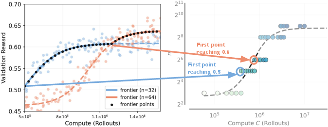
- They tried many combinations of , , and under the same total compute. To fairly compare runs, they tracked “record-breaking” checkpoints—the moments when a run first reached a new, higher score—and fit smooth curves to the best results (the “frontier”).
What did they find, and why does it matter?
Here are the key findings, explained with simple ideas. This list is meant to make the results easy to skim.
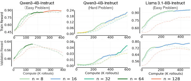
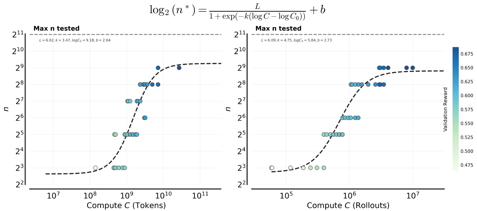
- The best number of tries per question () should grow as your compute budget grows, then level off.
- When you have more compute, spend more of it on trying multiple answers per question (higher ), not just training longer () or adding more different questions per batch ().
- But this doesn’t go on forever—after a point, increasing doesn’t help much and “saturates.”
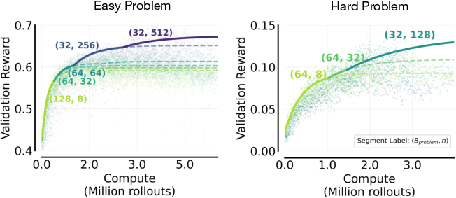
- Easy and hard questions both benefit from higher , but for different reasons:
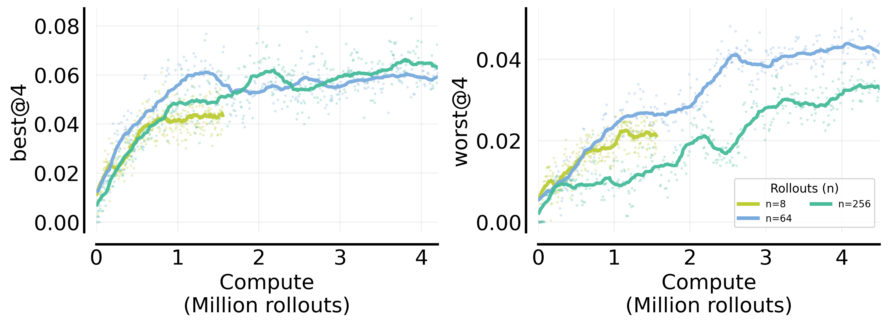
- Easy set: More tries per question mainly “sharpens” the model’s answers—many of its attempts become consistently right. This shows up in “worst@k” scores (all k answers are correct), which improve with higher .
- Hard set: More tries mainly boosts “coverage”—the chance that at least one attempt is right. This shows up in “best@k” scores (at least one of k answers is correct), which improve with higher .
- Translation: On easy stuff, more tries makes the model reliable; on hard stuff, more tries helps the model occasionally find a good path.
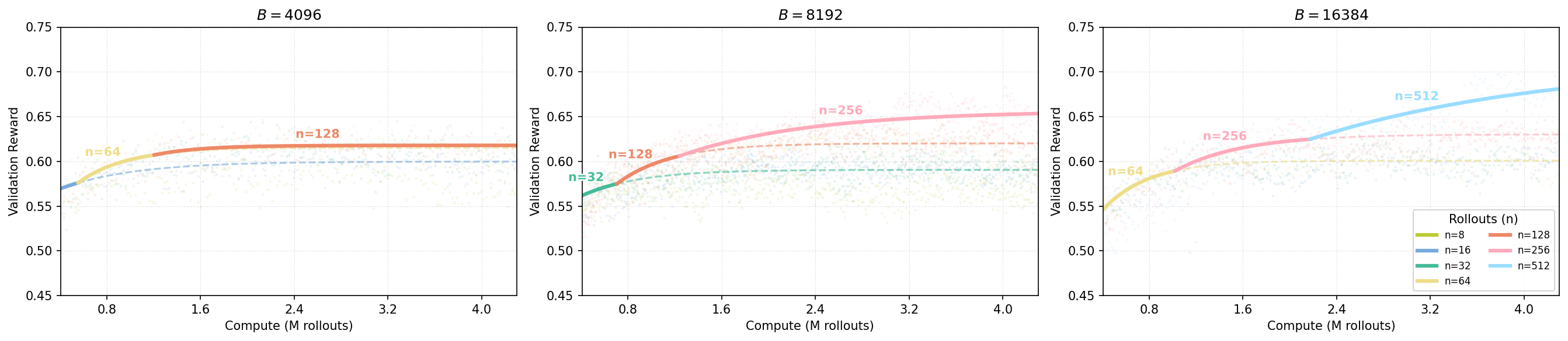
- If your hardware limits the total batch (), how you split it matters:
- With low overall training time ( small): Prefer more different questions ( bigger), fewer tries per question ( smaller). You need variety because you won’t revisit things much.
- With lots of training time ( large): Shift toward more tries per question ( bigger), fewer different questions per batch ( smaller). You’ll revisit questions enough times that deeper exploration per question pays off.
- On easy sets, performance barely changes across a broad range of , as long as it’s not extreme. matters much more.
- On hard sets, matters more than on easy sets and can affect stability, but still tends to be the more powerful lever.
- Why does increasing help so much? It reduces “interference” between questions.
- When you train on many different questions, learning on one can accidentally hurt another. More tries per question gives a clearer, more consistent signal for each question in each step, making progress more even and reducing this interference.
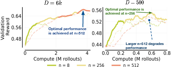
- These trends showed up across different base models and datasets, but the exact best depends on context.
- Bigger or stronger base models, smaller or harder datasets, and different difficulty mixes can change where stops helping (the saturation point).
What does this mean going forward?
The paper turns a fuzzy art—choosing training settings for RL on LLMs—into a clearer playbook:
- If you have a small compute budget:
- Use more different questions ( up), fewer tries per question ( down), and don’t expect to train for many steps ( modest).
- If you have a medium-to-large compute budget:
- Gradually increase tries per question ( up), and decrease how many different questions you bundle per step ( down), while allowing more training steps ( up).
- Match regularization to difficulty:
- Use entropy + KL (keep options open and stay close to the base model) for easy sets.
- Turn them off for hard sets to avoid instability and allow exploration.
- Use square-root learning-rate scaling with batch size for stability.
- Decide what you care about most:
- If you want high coverage (at least one correct out of several tries) on hard problems, lean more on .
- If you want high reliability (all tries correct) on easy problems, also helps.
In short, the authors provide simple, practical rules for how to spend your compute when doing RL with LLMs. Following these rules can make training more efficient, more stable, and better targeted to what you actually want—either broader coverage on hard tasks or more reliable answers on easier ones.
Knowledge Gaps
Knowledge gaps, limitations, and open questions
Below is a focused list of what remains missing, uncertain, or unexplored in the paper, phrased to guide follow‑up research.
- Scope limited to single‑turn, binary‑reward LLM RL:
- How do the allocation rules for , , and change for multi‑turn dialogue, multi-step reasoning, or tasks with sparse vs. dense, shaped, or continuous rewards?
- Algorithmic generality beyond on‑policy GRPO:
- The main results are for GRPO with brief mentions of PPO/CISPO in the appendix; do the compute‑optimal prescriptions hold for a wider class of on‑policy variants, off‑policy methods (e.g., replay buffers, value‑based RL), or hybrid RLHF pipelines?
- Theoretical underpinning of scaling laws:
- There is no formal derivation linking , , and to gradient variance/bias, interference across problems, or convergence; can a theory predict the sigmoidal , its saturation point, and when parallel vs. sequential compute should dominate?
- Dynamic/phase‑wise scheduling:
- The study treats , , as static per run; what time‑varying schedules (e.g., increasing late, curriculum‑aware , or adaptive ) are compute‑optimal across training phases?
- Per‑problem adaptive allocation:
- Can be allocated adaptively per prompt based on estimated difficulty, reward density, or uncertainty to reduce wasted sampling on persistently unsolved problems while avoiding overfitting?
- Dataset size and heterogeneity:
- The saturation of is attributed to fixed problem sets, but dataset size/composition is not systematically varied; how do scaling rules change under:
- Controlled increases in dataset size?
- Mixtures with varying skew, long tails, or shifting difficulty over time?
- Curricula that increase difficulty as the model improves?
- Task/domain coverage:
- Results are primarily on math (Guru‑Math) with easy/hard splits; do the conclusions transfer to code generation, instruction following, safety benchmarks, question answering, or multimodal tasks?
- Model scale and architecture:
- Only 4B–8B models are tested; how do saturation points and the – tradeoff evolve at 30B–70B–>100B+ models and across different architectures or decoding heads?
- Interference characterization and mitigation:
- Interference is inferred from pass@1 distributions, but mechanisms remain unclear; can we:
- Quantify interference with per‑problem gradient conflict metrics?
- Test mitigation strategies (e.g., per‑problem weighting, gradient surgery, multi‑task balancing, replay) and their effect on ?
- Regularization policies and stability:
- KL/entropy are toggled by difficulty, but broader regularization spaces (e.g., dynamic KL schedules, trust‑region constraints, length penalties) are not explored; what regularization schedules jointly maximize stability and performance across mixed‑difficulty datasets?
- Compute measurement and wall‑clock efficiency:
- Compute is measured in rollouts; token‑level compute and wall‑clock throughput (with varying lengths, batch packing, latency) are only briefly addressed; how do prescriptions change under token budgets or time/cost constraints?
- Frontier estimation methodology:
- The “record‑breaking point” and discretized binning approach may bias frontier estimation; how robust are results to alternative frontier fitting, noise models, or bootstrapped confidence intervals?
- Metric‑dependent optimality:
- The optimal differs for avg@k, best@k, and worst@k; how should practitioners choose when optimizing multi‑objective utility (coverage vs. robustness vs. calibration), and how do these choices affect downstream user experience?
- Off‑policy data reuse and replay:
- The study assumes fresh on‑policy samples; does replay (sample reuse) change the – tradeoff and the saturation behavior, especially under fixed compute?
- Response length and entropy dynamics:
- Length explosions and entropy collapse are noted qualitatively; what is the quantitative relationship between , regularization, response length distributions, and stability across easy/hard regimes?
- Reward noise and learned reward models:
- The main experiments use 0/1 outcome rewards with automatic correctness on math; how do the findings extend to noisy or learned reward models (RM‑based RLHF), where reward variance and bias differ?
- Generalization and regression:
- OOD results are limited; to what extent do compute‑optimal allocations that boost in‑domain metrics avoid overfitting and capability regression on unrelated tasks or safety benchmarks?
- Cross‑model difficulty splits:
- Easy/hard splits are defined using one base model’s pass@16; do conclusions hold when difficulty is defined per‑model, and how does the partitioning choice bias the observed scaling?
- Hardware and parallelism constraints:
- Different settings for easy vs. hard sets confound comparisons; how do recommendations change under standardized hardware constraints and diverse parallelization strategies (pipeline/model parallelism)?
- Interplay with test‑time compute:
- Training uses varying but evaluation uses fixed small (e.g., 4); how do training allocations interact with test‑time compute strategies (self‑consistency, majority voting, reranking) under fixed inference budgets?
- Broader hyperparameter space:
- Other critical knobs (optimizer types, clipping/coefficient schedules, advantage normalization schemes, truncation strategies) are held fixed; do compute‑optimal allocations persist across these choices?
- Safety and alignment considerations:
- Disabling KL on hard sets may enable capability gains but could increase drift from the base model; what are the safety implications and how should alignment constraints be integrated into compute‑optimal allocation?
- Reproducibility and variance:
- The impact of random seeds, dataset sampling noise, and run‑to‑run variance on the inferred frontiers and fits is not reported; what are confidence bands for the proposed prescriptions?
Practical Applications
Immediate Applications
The paper provides practical, prescriptive rules for compute allocation in LLM reinforcement learning (RL) post-training (on-policy, rollout-based methods such as GRPO/PPO). The following applications can be deployed now by engineering teams, researchers, and service providers.
- Compute-optimal RL job configuration and scheduling (Industry: software/ML infrastructure; Cloud)
- Use the playbook to choose rollouts per problem n, problems per batch B_p, and update steps M under a fixed rollout compute budget C = B_p * n * M.
- Workflow:
- At low compute budgets, favor larger B_p (smaller n) to increase coverage over problems; as compute increases, shift toward larger n (smaller B_p) to reduce gradient variance and mitigate interference.
- Tune learning rate with square-root scaling relative to total batch size (η ∝ √B where B = B_p * n).
- Under fixed hardware (max batch B), increase n with training progress (M) on easy datasets; maintain a minimal stable B_p.
- Tools/products:
- Job templates for Ray/SLURM/Lightning; Azure/AWS “compute-optimal RL” presets; config generators that output (n, B_p, M) from a budget and dataset profile.
- Assumptions/dependencies: On-policy rollout RL; binary or programmatically scored rewards; single-turn settings; stable training recipe (KL+entropy for easy data, no KL/entropy for hard data).
- Cost and ROI forecasting for RL post-training (Industry/Finance; Cloud FinOps)
- Use the observed sigmoidal scaling of n*(C) and frontier fitting (record-breaking checkpoint method) to forecast incremental benefits of more compute and identify saturation points.
- Workflow: Early small-budget runs → fit compute–reward frontier → extrapolate expected gains at target budget.
- Assumptions/dependencies: Base-model-, dataset-, and metric-specific; requires a small pilot sweep to calibrate.
- Interference-aware training and monitoring (Industry: ML engineering; Safety)
- Monitor training-set pass@1 distributions to detect uneven learning or capability erosion across problems; increase n to reduce interference and make updates more uniform.
- Tools/products: Training dashboards tracking pass@k histograms, best@k vs worst@k; alarms when zero-pass fraction rises.
- Assumptions/dependencies: Per-problem evaluation at train time; stable logging; fixed or slowly drifting data mixture.
- Metric-aligned training strategies (Industry: product ML; Safety)
- Align n to business targets:
- If coverage (best@k/pass@k) is the objective on hard problems, prefer larger n.
- If robustness (worst@k) is the objective on easy problems, prefer larger n; for coverage on easy problems, smaller n can suffice.
- Tools/products: “Coverage vs sharpening” switch in training configs; metric-aware hyperparameter schedulers.
- Assumptions/dependencies: Clear product metric hierarchy; consistent evaluation pipeline; k chosen well below n.
- Difficulty-aware RL recipes and data curation (Industry/Academia; Healthcare/Legal/Code models)
- Partition datasets into “easy” and “hard” using base model avg@k (e.g., avg@16) and apply matching regularization:
- Easy: enable KL + entropy to prevent entropy collapse.
- Hard: disable KL + entropy to avoid instability and length explosion.
- Tools/products: Data curation scripts that compute avg@k; auto-assign recipes; curriculum builders.
- Assumptions/dependencies: Reliable programmatic judge for reward; base model reasonably competent to estimate difficulty.
- Standardized experimental protocols and reporting (Academia; Open-source)
- Adopt record-breaking checkpoint selection to avoid bias when fitting compute frontiers; report (n, B_p, M, B_max), difficulty splits, and learning-rate scaling.
- Tools/products: Repro templates; logging schemas; benchmark leaderboards that separate easy vs hard subsets.
- Assumptions/dependencies: Comparable reward definitions; shared validation splits.
- Plug-and-play “IsoCompute Scheduler” library (Industry/Academia/Open-source)
- A small utility that:
- Takes budget C, hardware B_max, base model size, dataset difficulty stats.
- Outputs recommended (n, B_p, M) and LR scaling; updates n*(C) schedule as training progresses.
- Integration targets: PyTorch Lightning, TRL, Ray Tune, vLLM-based samplers, Hydra configs.
- Assumptions/dependencies: Pilot sweep data to fit initial sigmoid; adherence to the stable recipe.
- RL post-training services and SLAs (Cloud/Consulting)
- Offer “compute-optimal RL” as a managed service with explicit trade-offs and milestones (coverage vs robustness).
- Tools/products: Budget-to-metric dashboards; carbon/energy estimates aligned with compute frontiers.
- Assumptions/dependencies: Access to datasets, graders, and customer-defined metrics; credits/budget constraints.
- MLOps runbooks for stability (Industry)
- Canonical runbooks: square-root LR scaling; KL/entropy toggles by difficulty; minimum stable B_p thresholds; maximum n per context (saturation); token length monitoring on hard sets.
- Assumptions/dependencies: Known instability modes (entropy collapse/explosion); monitoring hooks.
- Sector-specific domain models (Healthcare/Education/Finance/Code)
- Apply the playbook to domain RL pipelines where binary or programmatic signals exist (e.g., unit tests for code, rubric checks for math/logic).
- Expected benefit: Faster time-to-target pass@k at lower cost.
- Assumptions/dependencies: High-quality auto-graders; domain-appropriate constraints (e.g., safety guardrails in healthcare).
- Sustainability and compute-efficiency policies (Policy/ESG; Industry governance)
- Use compute-optimal allocation to minimize wasted sampling compute; report energy/carbon for chosen frontier operating points.
- Tools/products: Compute disclosures, carbon dashboards; procurement guidelines that prefer runs near saturation points.
- Assumptions/dependencies: Energy metering; organization-level sustainability goals.
- Education and training materials (Academia/Education)
- Course modules demonstrating scaling laws, interference, and compute allocation decisions; lab assignments using open models/datasets.
- Assumptions/dependencies: Access to modest compute; open benchmarks with programmatic rewards.
Long-Term Applications
These opportunities require additional research, engineering, or ecosystem development (e.g., beyond single-turn, binary rewards; broader generalization; automation).
- Closed-loop, adaptive controllers for n, B_p, M (Industry/Cloud; AutoML)
- Online tuning that adjusts n and B_p in real time based on learning progress, interference metrics, and target metrics (best@k vs worst@k).
- Tools/products: “RL Autopilot” atop Ray/Lightning; Bayesian optimization with scaling-law priors.
- Dependencies: Robust live metrics; stability under frequent hyperparameter changes; safe rollback.
- Interference-aware curricula and routing (Industry/Academia)
- Cluster problems by gradient similarity; assign per-cluster n; or use mixture-of-experts and problem routing to reduce cross-problem interference.
- Dependencies: Efficient gradient/statistics collection; theory-guided interference estimators; scalable clustering.
- Generalized scaling laws (Academia/Industry)
- Extend prescriptions to multi-turn RL, non-binary and learned rewards, off-policy methods, and domains beyond reasoning (e.g., tool use, planning).
- Dependencies: Datasets with reliable long-horizon reward; multi-turn judges; algorithmic stability advances.
- Energy- and token-aware scheduling (Cloud/Policy)
- Replace rollout-count proxies with token-level, energy-metered compute models for scheduling and reporting; optimize for both cost and carbon.
- Dependencies: Accurate token-length prediction; standardized energy telemetry across hardware.
- Safety-aligned coverage/robustness dashboards (Industry/Regulated sectors)
- Mature product instrumentation for “coverage vs sharpening” trade-offs tied to safety/hallucination metrics; automated guardrails adjusting n to enforce reliability thresholds.
- Dependencies: Calibrated judges; sector-specific risk models; compliance integration.
- Data–compute co-optimization policies (Industry/Procurement/Policy)
- Decide when to acquire more data vs allocate more compute per problem (RL “Chinchilla-like” rules for data size vs n/M); inform data valuation and procurement.
- Dependencies: Learning curves across dataset scales; standardized data difficulty measures; cost models.
- Standardization and governance (Policy)
- Best-practice standards for reporting (n, B_p, M), difficulty splits, regularization choices, and compute frontiers in RL training publications and audits.
- Dependencies: Community consensus; support from conferences, regulators, and cloud providers.
- Automated difficulty estimation pipelines (Industry/Academia)
- Continuous labeling of problem difficulty (e.g., rolling avg@k) to select recipes and target n adaptively as models improve.
- Dependencies: Reliable and cheap programmatic evaluation; drift detection.
- Cross-domain agent training and test-time compute policies (Robotics/Software agents)
- Translate training-time insights to test-time policies for allocating rollouts per task instance (balancing coverage vs reliability within latency/compute budgets).
- Dependencies: Task-time constraints; online judges; alignment with product latency SLAs.
- Multi-tenant cluster optimization (Cloud/MLOps)
- Fair-share schedulers that assign batch budgets and recommended n to concurrent RL jobs to keep each near its compute-optimal frontier.
- Dependencies: Job characterization APIs; isolation and fairness policies.
- Carbon-aware SLAs (Cloud/ESG)
- Offer SLAs that guarantee target pass@k within both monetary and carbon budgets using compute-optimal scheduling.
- Dependencies: Metered carbon intensity; geographic scheduling; customer acceptance.
- Theory-informed resource allocation (Academia)
- Formal models linking interference, gradient covariance, and optimal n/B_p trade-offs; principled criteria for saturation detection and stopping rules.
- Dependencies: New analytical tools; validated simulators and empirical benchmarks.
Notes on Assumptions and Dependencies (global)
- Method scope: On-policy, rollout-based RL (e.g., GRPO/PPO), largely single-turn, binary outcome rewards; results generalize qualitatively across several base models but require calibration.
- Stability prerequisites: Square-root LR scaling with batch size; regularization policy (KL+entropy for easy, none for hard); zero-variance filtering not required but affects stability.
- Context sensitivity: Optimal n saturates and depends on base model capacity, dataset size, and difficulty; pilot runs are needed to estimate saturation.
- Metrics matter: Compute-optimal choices differ if optimizing for avg@k, best@k (coverage), or worst@k (robustness).
- Infrastructure: Requires scalable sampling and logging; reliable programmatic judges; hardware constraints (B_max) shape feasible allocations.
Glossary
- avg@16: A difficulty proxy measuring a base model’s average accuracy over 16 rollouts on a problem. "We quantify difficulty by avg@16, the base modelâs average accuracy over 16 rollouts"
- best@k: Coverage metric; fraction of problems where at least one of k sampled responses is correct. "best@k (or pass@k), defined as the fraction of problems where {at least one} response out of is correct"
- CISPO: An RL algorithm variant related to PPO/GRPO used for policy optimization. "this qualitative trend is not specific to the GRPO algorithm considered here, and appears under other algorithmic variants~(PPO~\cite{schulman2017proximal} and CISPO~\cite{minimax2025minimaxm1scalingtesttimecompute}) as well"
- compute budget: The total amount of allowable compute (here, sampling) for an experiment. "optimal number of rollouts increases with the compute budget "
- compute-optimal frontier: The curve of best achievable validation performance for a given compute amount. "we define the compute-optimal frontier as the highest i.i.d. validation set reward achievable using total compute "
- coverage: The breadth of distinct problems for which the model can produce at least one correct solution. "leading to gains in best@k and improved coverage."
- coverage expansion: Mechanism where more rollouts discover rare successful trajectories on hard problems. "solution sharpening on easy problems and coverage expansion on hard problems."
- data-parallel: Parallelization across devices/tasks to increase batch throughput. "hardware parallelism (e.g., number of GPUs or data-parallel) is fixed"
- effective batch size: Total number of samples contributing to a single gradient update. "The effective batch size per iteration is "
- entropy bonus: A regularizer that encourages exploration by rewarding higher policy entropy. "Hence, whenever we employ an entropy bonus, we pair it with a KL anchor."
- entropy regularization: Adding an entropy term to the loss to prevent premature collapse and sustain exploration. "we apply both KL and entropy regularization on easy problem sets"
- entropy collapse: Failure mode where policy entropy drops too quickly, reducing exploration and learning. "On easy problems, insufficient entropy regularization often leads to premature entropy collapse"
- GRPO: A rollout-based on-policy RL method using grouped normalization of advantages. "rollout-based on-policy algorithms such as GRPO~\citep{arxiv-org-2402-03300-2}, which generate multiple rollouts per prompt and optimize the policy using group-normalized advantages."
- group-normalized advantages: Advantage estimates normalized within each prompt’s rollout group to stabilize updates. "optimize the policy using group-normalized advantages."
- hardware-driven batch size constraint: A limit on batch size imposed by available compute hardware. "we additionally incorporate a hardware-driven batch size constraint "
- i.i.d. validation set: A validation set assumed independently and identically distributed relative to the training distribution. "the highest i.i.d. validation set reward achievable using total compute "
- interference: Gradient conflict across different problems leading to uneven learning or regressions. "increasing the number of parallel rollouts mitigates interference across problems"
- KL anchor: A KL penalty term that tethers the policy to a reference model to prevent drift. "we pair it with a KL anchor."
- KL divergence: Regularizer measuring divergence from a reference policy to control drift. "Factor 2: Entropy and KL-divergence regularization."
- learning-rate scaling: Adjusting the learning rate as a function of batch size to maintain stable optimization. "Factor 3: Learning rate scaling."
- monotonic function: A non-decreasing fit used to model performance frontiers without spurious reversals. "We then fit a monotonic function to these record-breaking points"
- multi-armed bandit: A simplified decision-making setting illustrating exploration–exploitation trade-offs. "If we were given a multi-armed bandit problem, in a tabular setting, the compute-optimal scaling strategy would prescribe increasing "
- OOD (out-of-domain): Data or tasks outside the training distribution used to assess generalization. "We also show scaling improves not only in-domain validation, but also OOD downstream tasks"
- on-policy RL: Reinforcement learning where data is collected using the current policy being optimized. "We study the compute-optimal allocation of sampling compute for on-policy RL methods in LLMs"
- pass@k: Probability that at least one of k sampled solutions per problem is correct. "best@k (or pass@k), defined as the fraction of problems where {at least one} response out of is correct"
- policy-gradient variance: Variability in gradient estimates from stochastic policy sampling; reduced by more rollouts. "increasing lowers policy-gradient variance"
- PPO: Proximal Policy Optimization, a widely used on-policy RL algorithm. "appears under other algorithmic variants~(PPO~\cite{schulman2017proximal} and CISPO~\cite{minimax2025minimaxm1scalingtesttimecompute}) as well"
- prompt distribution: The distribution over input problems/prompts used during training/evaluation. "scaling behavior in RL is governed not only by total compute, but also by the interaction between the base model and the prompt distribution."
- record-breaking points: Checkpoints that exceed all previous validation rewards along a run. "A record-breaking point is the earliest step at which the validation reward exceeds all previously observed values"
- rejection fine-tuning: Training using only accepted samples (e.g., high-quality generations) from a larger set. "cannot overcome limitations imposed by a fixed problem set for rejection fine-tuning."
- response-length explosion: Instability where generated outputs become excessively long during training. "entropy regularization alone can trigger entropy and response-length explosion"
- RL post-training: Reinforcement learning applied after base pre-training to further align/improve LLMs. "scaling laws for RL post-training of LLMs"
- sampling compute: Compute spent on generating rollouts/samples during RL training. "the primary resource constraint is sampling compute, which is proportional to the total number of generated rollouts"
- sequential iterations (M): The number of sequential gradient update steps in training. "and sequential iterations ()"
- sigmoidal behavior: S-shaped scaling pattern of performance versus resources. "RL reward curves exhibit clean sigmoidal behavior"
- solution sharpening: Mechanism where training improves robustness/consistency on already solvable problems. "solution sharpening on easy problems and coverage expansion on hard problems."
- square-root scaling: Learning-rate scaling rule proportional to the square root of batch size. "square-root scaling () provides the best trade-off"
- system batch size: The largest batch saturating throughput on available hardware. "B is often chosen as the largest rollout batch size that saturates sampling throughput (\"system batch size\")."
- upper envelope: The pointwise maximum across fitted curves used to define a performance frontier. "we then define the compute-optimal frontier as the upper envelope of these fitted curves"
- worst@k: Robustness metric; fraction of problems where all k sampled responses are correct. "worst@k, defined as the fraction of problems where all responses are correct"
- zero-variance filtering: A stabilization technique that filters regularizers when variance is near zero. "While applying zero-variance filtering~\citep{arxiv-org-2510-13786} to these terms mitigates instability"
Collections
Sign up for free to add this paper to one or more collections.