On the Role of Batch Size in Stochastic Conditional Gradient Methods
Abstract: We study the role of batch size in stochastic conditional gradient methods under a $μ$-Kurdyka-Łojasiewicz ($μ$-KL) condition. Focusing on momentum-based stochastic conditional gradient algorithms (e.g., Scion), we derive a new analysis that explicitly captures the interaction between stepsize, batch size, and stochastic noise. Our study reveals a regime-dependent behavior: increasing the batch size initially improves optimization accuracy but, beyond a critical threshold, the benefits saturate and can eventually degrade performance under a fixed token budget. Notably, the theory predicts the magnitude of the optimal stepsize and aligns well with empirical practices observed in large-scale training. Leveraging these insights, we derive principled guidelines for selecting the batch size and stepsize, and propose an adaptive strategy that increases batch size and sequence length during training while preserving convergence guarantees. Experiments on NanoGPT are consistent with the theoretical predictions and illustrate the emergence of the predicted scaling regimes. Overall, our results provide a theoretical framework for understanding batch size scaling in stochastic conditional gradient methods and offer guidance for designing efficient training schedules in large-scale optimization.
Paper Prompts
Sign up for free to create and run prompts on this paper using GPT-5.
Top Community Prompts
Explain it Like I'm 14
Overview
This paper asks a simple, practical question about training big LLMs (like GPT): if you have a fixed “token budget” (a limit on how many words/subwords you can process during training), how should you choose batch size, sequence length, and learning-rate-like settings to learn as well as possible?
The authors study a family of optimizers called stochastic conditional gradient (SCG) methods (used in modern “projection‑free” optimizers) and show how batch size interacts with learning rate, noise, and the fixed token budget. They discover clear “scaling rules” that tell you when making batches bigger helps, when it stops helping, and when it actually hurts—plus how to set the learning rate to match. They test these ideas on NanoGPT and find that the theory matches what they see in practice.
Key questions
In simple terms, the paper tries to answer:
- If you can only see a fixed number of tokens during training, how big should your batch size and sequence length be?
- How should you set the step size (think: a learning-rate-like parameter) to make the most progress with your token budget?
- When does increasing batch size help, and when does it stop helping—or even make things worse?
- Can we design a simple, stage‑wise schedule to change batch size and step size during training that keeps things efficient?
Approach (what they did, explained simply)
Think of training as climbing down a bumpy hill (the loss surface) to the bottom (good performance). At each step, you decide which direction to move and how big a step to take.
- Optimizer studied: SCG (stochastic conditional gradient).
- Instead of taking a step and then “projecting” back into a safe region (which can be expensive), SCG picks a direction that already stays within the allowed limits. You can imagine asking a helper, “Within the rules, which way points most downhill?” and stepping that way.
- Momentum is used to smooth out noisy directions across steps, like averaging recent compass readings so you don’t overreact to random gusts of wind.
- Token budget: You only have T tokens to spend. Each training update processes B sequences, each of length S, so one update uses BS tokens. That means the number of updates K you can take is K = T / (B·S). Larger batches and longer sequences use up your budget faster, so you get fewer updates.
- Noise and curvature: The paper assumes two realistic facts that are also seen in practice:
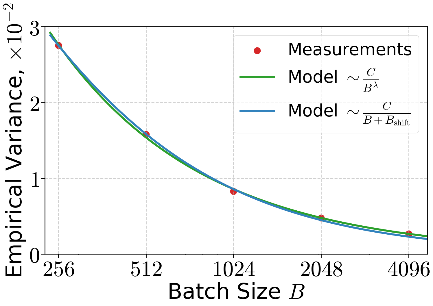
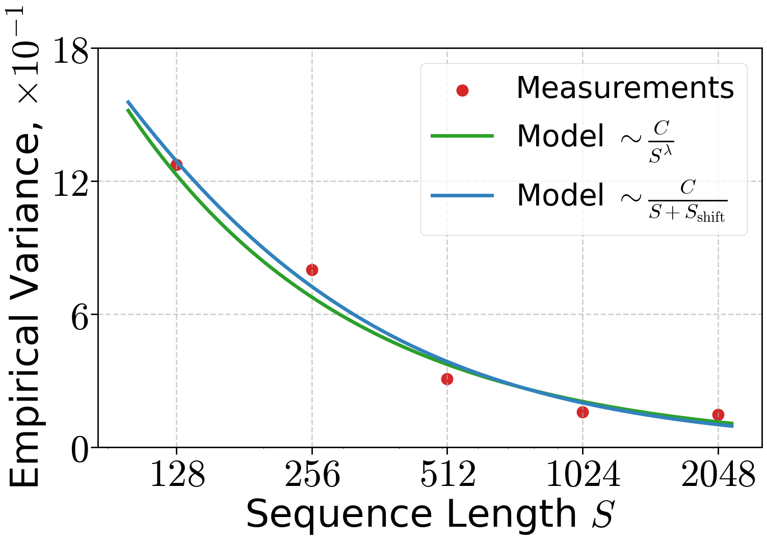
- Gradient noise shrinks when you use a bigger batch and/or longer sequences, roughly like 1/(B·S). Bigger batches average out randomness.
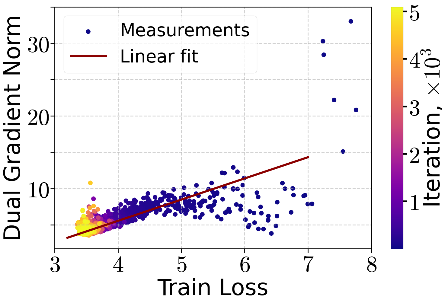
- There’s a relationship between how steep the hill is and how far you are from the bottom (a “KL condition”). Think: if the slope is big, you’re far from the bottom; if it’s small, you’re closer. The authors check this on NanoGPT and see it holds well after the loss drops below a certain value.
- Analysis strategy: Write down how the training error depends on:
- how many updates you make (K),
- how big and long your batches are (B and S),
- your step size (a Frank–Wolfe step parameter they call β),
- and the noise level.
- Then solve for the best trade‑offs when T (the total tokens) is fixed.
Main findings (what they discovered and why it matters)
Here are the core takeaways, explained with minimal math:
- Three training regimes under a fixed token budget
- Small effective batch (BS is small): Increasing BS helps because it reduces noise. Training gets more accurate.
- Middle regime: Past a certain point, increasing BS doesn’t change the final accuracy much. It’s flat with respect to BS.
- Very large effective batch (BS is big): Increasing BS starts to hurt because you run out of updates (K = T/(BS) gets too small). Accuracy gets worse.
- A simple “BST scaling rule” for best overall efficiency
- The sweet spot comes from balancing the middle and large‑batch effects. The result is a clear scaling rule for the product of batch size and sequence length:
- This means: for a larger token budget T, you should grow the effective batch (B times S) like , not linearly.
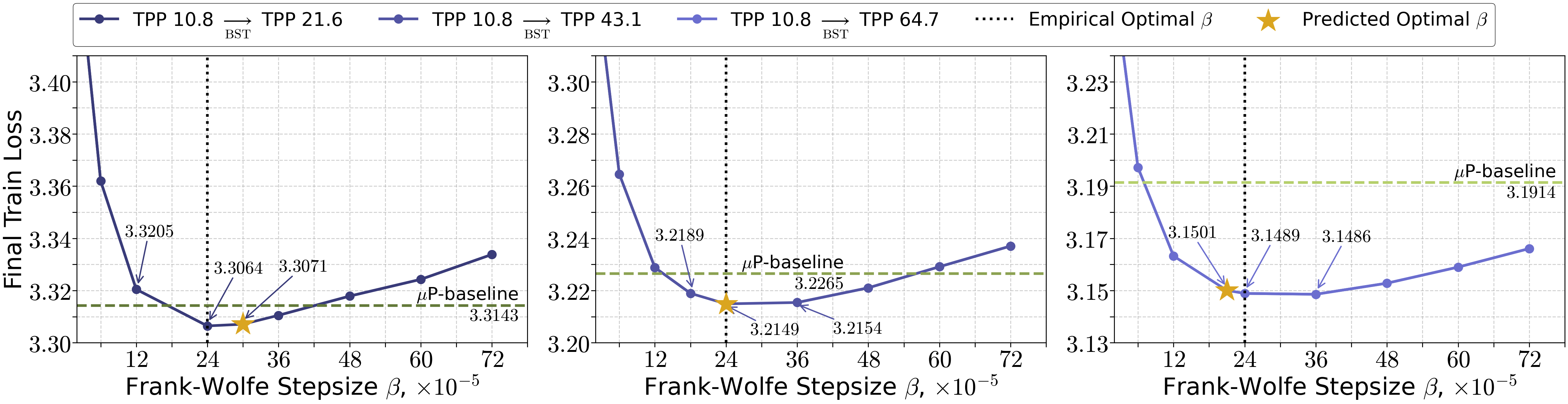
- How to set the step size
- The analysis says the Frank–Wolfe step parameter should scale like:
- In words: make β roughly inversely proportional to the number of updates. If you take fewer updates (because BS is larger), increase β accordingly, and vice versa.
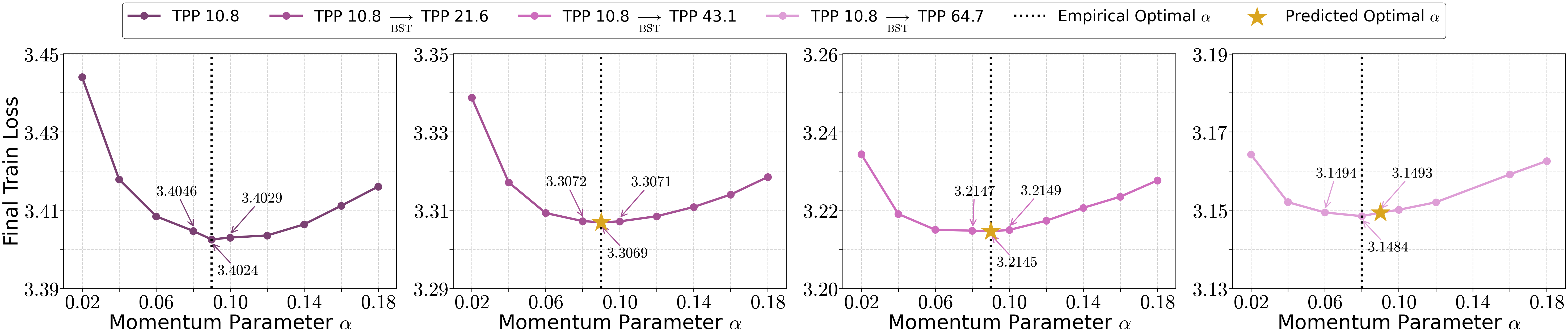
- Momentum can stay roughly constant
- Under the proposed scaling, the momentum parameter doesn’t need to change much across sizes. That’s convenient: once you find a good momentum setting, you can often keep it.
- A practical, stage‑wise schedule
- If you train in stages (for example, more data arrives later), you can:
- start with smaller BS,
- then increase BS following as your total token budget grows,
- and adjust β in step with the total number of updates ().
- This preserves both convergence and efficiency as the training horizon grows.
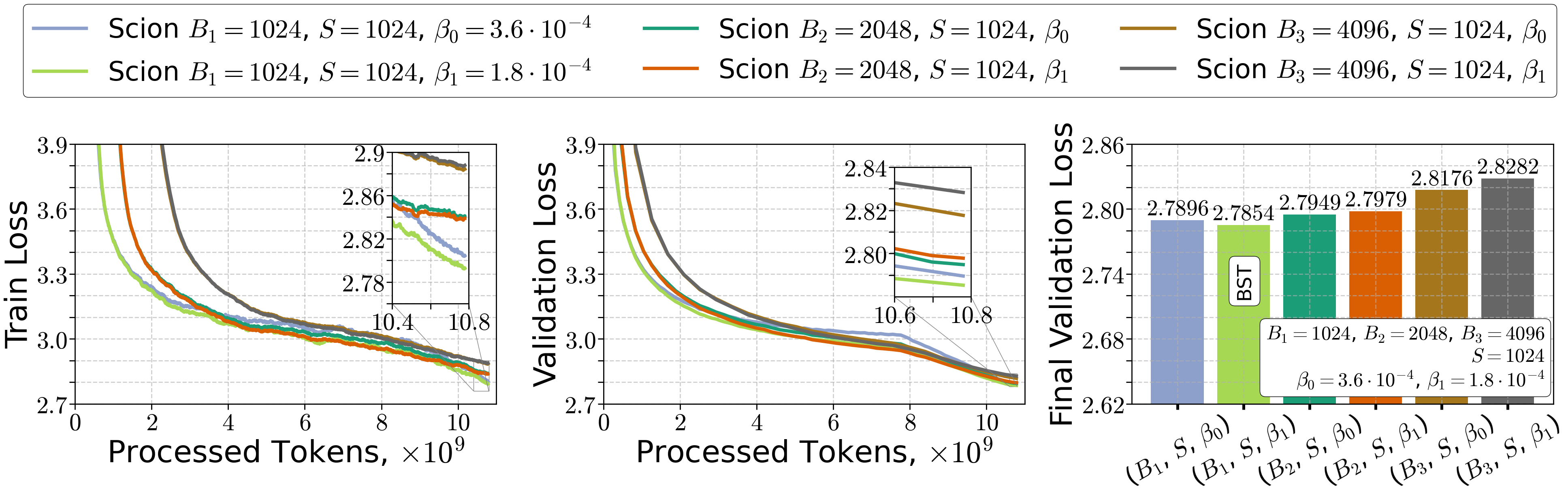
- Experiments match the theory
- On NanoGPT with a real dataset, they observe:
- Gradient noise indeed falls roughly like 1/(B·S).
- The “KL condition” (gradient size relates to how far you are from the bottom) holds well in later training.
- The three regimes show up in practice: increasing BS helps, then plateaus, then hurts if you push it too far under a fixed token budget.
- Using the scaling rules leads to sensible, efficient choices of batch size, sequence length, and step size.
Why this matters
- Better use of compute: If you have a fixed budget of tokens, this tells you how to turn that budget into the most useful progress by choosing batch size, sequence length, and step size wisely.
- Clarity on “large batch hurts”: Large batches aren’t bad by themselves. They become bad only if you don’t adjust the learning‑rate‑like step size and the number of updates correctly under a fixed token budget. Follow the scaling rules, and large batches can still be efficient.
- Simple, portable rules: and are easy to remember and implement. Momentum can stay about the same.
Practical rules you can apply
If you plan training with a fixed total number of tokens T:
- Choose batch size and sequence length so their product scales like .
- Set the step parameter roughly like where .
- Keep momentum about the same across runs; tune it once and reuse it.
These guidelines help you avoid wasting tokens on too many tiny updates or too few giant updates and keep your training both stable and efficient as you scale up.
Knowledge Gaps
Knowledge gaps, limitations, and open questions
Below is a consolidated list of what remains uncertain or unexplored in the paper, framed to guide concrete follow-up work.
- Validity and scope of the μ-KL assumption:
- Formal conditions under which μ-KL holds for transformer training in Scion/SCG geometry are not established; empirical support is limited to a single 124M NanoGPT run and a subset of the loss range (loss ≲ 5). How μ varies across training stages, datasets, architectures, and norm choices remains unknown.
- Estimation and evolution of problem-dependent constants (L, μ, ρ, σ∗):
- No practical, robust procedure is provided to estimate these constants online at scale or to track how they evolve with model size, batch size, sequence length, and training progression. The proposed use of fitted power laws is not operationalized for production settings.
- Noise model realism:
- The bounded-variance assumption σ² ≍ σ∗²/(BS) is idealized. Observed exponents deviate from 1 and exhibit shifts; the model ignores token/token correlations within sequences, gradient accumulation effects, mixed precision/quantization noise, and potential heavy-tailed or nonstationary noise. A more realistic, stage- and sequence-length–aware noise model is needed.
- Role of sequence length S beyond variance scaling:
- The analysis treats S only via variance reduction and token budgeting, neglecting that transformer compute and memory scale superlinearly with S (e.g., attention O(S²)) and that larger S alters curvature and optimization dynamics. A compute-budget–aware scaling law and a model of how S affects L and μ are missing.
- Optimization-to-generalization connection:
- Results bound optimization error only; they do not explain when/why large batches hurt generalization beyond iteration-starvation. A theory linking SCG geometry, batch size, sharpness/flatness, and test performance is absent.
- Optimizer mismatch and transferability:
- The BST rule is derived for SCG/Scion; most LLMs use AdamW or variants. It remains open whether the BS ∝ T{2/3} and β ∝ 1/K prescriptions transfer to Adam-like optimizers theoretically or empirically (or how to translate them into Adam hyperparameters).
- Momentum parameter α:
- The theorem prescribes α as a function of ε and σ, while the practical guideline claims α can be held constant across scales. The conditions under which a constant α is near-optimal, and how α should adapt to changing noise/curvature, are not characterized or validated.
- Choice of LMO radii η and layerwise geometry:
- Radii are set heuristically (e.g., 3000/50) without sensitivity analysis or guidance on how η influences L, μ, ρ and the scaling rule. A procedure to set/adjust η per layer (and its effect on guarantees) is lacking.
- Adaptive/online scheduling without known T:
- The proposed schedules assume the final token budget T is known. Practical algorithms to adapt B, S, and β online when T is uncertain (e.g., delayed-data or streaming settings) using observable signals (e.g., noise scale, gradient norms) are not developed.
- High-probability and sharp non-asymptotic guarantees:
- Convergence is analyzed in expectation with hidden constants/log factors. High-probability bounds with explicit constants are needed to predict practical regime transitions and to calibrate the “critical BS” threshold.
- Scale and data diversity of empirical validation:
- Experiments are limited to a single 124M model, one dataset (FineWeb), and few budgets/settings. Verification of the three regimes and the BS ∝ T{2/3} law across model scales (≥1B parameters), diverse corpora, and broader T is missing.
- Time-varying and stage-dependent constants:
- The theory does not model how L, μ, ρ, and σ evolve during training (e.g., with loss reduction or curriculum), though empirical CBS is known to be stage-dependent. A dynamic theory with time-varying constants and stage-aware schedules is needed.
- Compute/memory and systems constraints:
- Hardware constraints (GPU memory, throughput, pipeline parallelism), microbatching, and gradient accumulation staleness are ignored in the scaling rule. Integrating per-step wall-clock costs, memory limits, and distributed training effects into the BS/S schedule remains open.
- Alternative smoothness regimes:
- Extending the analysis beyond global L-smoothness to generalized/relative or local smoothness (e.g., (L0,L1)-smoothness) and to composite/non-smooth objectives is left to future work and remains a gap.
- Optimality and lower bounds:
- It is unknown whether the ε ≍ T{-1/3} rate and BS ≍ T{2/3} scaling are minimax-optimal for SCG under μ-KL. Lower bounds or tightness results would clarify optimality and the potential for improved algorithms.
- Geometry and norm choices:
- How the norm-equivalence constant ρ (and thus the scaling rule) depends on the chosen layerwise norms and alternative LMO geometries (e.g., path norms, spectral vs. other operator norms) is unquantified. Guidance on geometry selection to improve constants is absent.
- Practical estimation of σ∗ at scale:
- The variance estimation procedure (multiple mini-batch gradients per step) is expensive. Low-overhead, reliable online estimators of the noise scale suitable for large-scale training are not provided.
- Early training and warmup:
- μ-KL appears not to hold early in training. When and how to transition from warmup to BST-driven scheduling, and how to design stage-wise schedules that respect changing regimes, are not specified or validated.
- Interaction with common LR schedules and regularization:
- The β ∝ 1/K guidance is not reconciled with widely used cosine/step LR schedules, AdamW decoupled weight decay, or gradient clipping. A combined schedule compatible with practical training recipes is not derived.
Practical Applications
Immediate Applications
The following applications can be deployed now using the paper’s findings, with light engineering effort in standard ML stacks (e.g., PyTorch, DeepSpeed, HuggingFace Accelerate).
- Token-budget–aware batch–sequence scheduling for LLM training (sectors: software/AI infrastructure, cloud)
- What: Choose batch size B, sequence length S, and stepsize β to satisfy the BST scaling rule BS ≍ T2/3 and β ≍ 1/K under a fixed token budget T=K·B·S. Use the crossover regime to avoid iteration-starved large batches.
- Tool/workflow: “BST Scheduler” callback for PyTorch/DeepSpeed that automatically sets and updates (B, S, β) from the training budget, respecting memory limits and hardware throughput.
- Assumptions/dependencies: SCG/Scion- or Muon-like (projection-free, norm-constrained) optimizers; approximate μ-KL behavior and σ2∝1/(B·S); capacity to measure/estimate L, μ, ρ (or use defaults); availability of sufficiently long sequences if S increases; GPU memory headroom.
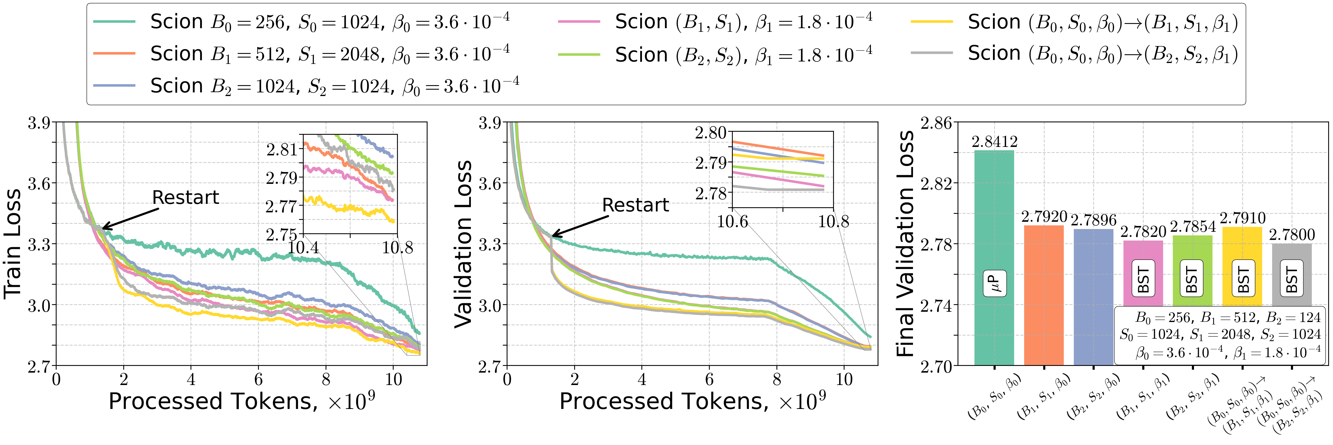
- Two-stage (and multi-stage) training when data arrives over time (sectors: software/AI infrastructure, data platforms)
- What: Start large-model training with early token budget T(1), then “restart” hyperparameters when additional tokens T(2) arrive, scaling (B·S) and β to the final T(1)+T(2) per the BST rules.
- Tool/workflow: Training orchestration that implements stage transitions (checkpoint → adjust B, S, β → resume).
- Assumptions/dependencies: Same as above; reliable tracking of processed tokens; restart-safe optimizer state.
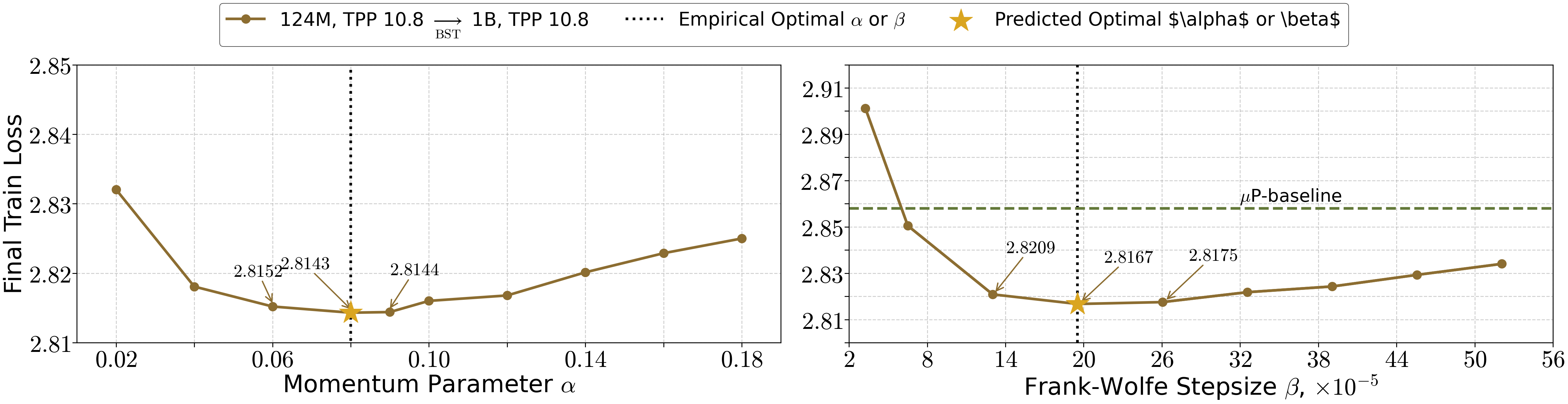
- Hyperparameter transfer from small to large models or from small to large token budgets (sectors: industry labs, academia)
- What: Reuse tuned (B0, S0, β0) from a small model or smaller T and transfer to a larger model or larger T using the paper’s scaling formulas for (B1·S1) and β1; keep momentum α constant.
- Tool/workflow: Lightweight “HP-Transfer” script that consumes source and target (T, model size, estimated L, μ, ρ) and emits target (B, S, β).
- Assumptions/dependencies: Estimating or holding constant L, μ, ρ; μ-KL and bounded-variance approximations; sufficient memory for increased S.
- Online diagnostics to prevent harmful large-batch regimes (sectors: software/AI infrastructure, MLOps)
- What: Monitor dual gradient norms vs loss to estimate μ, and empirical variance vs (B, S) to check σ2∝1/(B·S). Use a “regime indicator” to avoid the iteration-starved region where error grows with B·S.
- Tool/workflow: Training dashboard that logs and fits power laws for variance and KL slope; emits alerts when crossing regime boundaries.
- Assumptions/dependencies: Access to per-step gradient statistics; minor overhead for logging and fitting.
- Efficient fine-tuning under fixed data budgets (sectors: healthcare, finance, law)
- What: For domain LLM fine-tuning with limited tokens, use BST scheduling to maximize token efficiency and avoid large-batch degradation; choose β ≍ 1/K and keep α constant.
- Tool/workflow: “Budget-Aware Fine-Tuning” recipes integrated into standard fine-tuning pipelines.
- Assumptions/dependencies: Data privacy/compliance constraints restrict tokens; SCG-like optimizer availability; long-context data if S grows; careful monitoring of generalization.
- Compute and cloud cost planning (sectors: cloud, enterprise MLOps)
- What: Use ε ≍ max{ L·B·S/(μ2·T), (L·ρ2·σ*2/(μ4·T))1/3, ρ·σ*/(μ·(T2·B·S)1/6) } to translate token budgets into expected optimization error and select budget-aware (B, S, β).
- Tool/workflow: Spreadsheet or web calculator for “token-to-loss planning” that recommends (B, S, β) given T and constraints.
- Assumptions/dependencies: Rough constants (L, μ, ρ, σ*) from small pilot runs; the error law is optimization-side (separate from irreducible/generalization error).
- Federated/edge training with token quotas (sectors: mobile/edge, federated learning)
- What: Per-client adaptation of (B, S, β) to local token budgets and memory; server coordinates BST-compliant global schedule.
- Tool/workflow: FL server plugin that negotiates BST parameters per round.
- Assumptions/dependencies: Heterogeneous devices and sequence-length limits; stable SCG/LMO implementations on devices.
- Robust norm-constrained training for safety-critical models (sectors: autonomous systems, healthcare)
- What: Combine spectral/operator norm constraints (LMO geometry) with BST scheduling to stabilize training and bound updates without projections.
- Tool/workflow: Scion/Muon-style training recipes prepackaged for safety-relevant deployments.
- Assumptions/dependencies: Correct choice of layer-wise norms and radii; potential throughput trade-offs from LMO calls.
- Education and research reproducibility (sectors: academia, education)
- What: Course modules and lab assignments on token-budget–aware scaling; standardized reporting of (B, S, T), regime identification, and BST compliance.
- Tool/workflow: Teaching notebooks demonstrating μ-KL verification and variance fitting; open-source recipes for NanoGPT-like models.
- Assumptions/dependencies: Public datasets; small GPU access; consistent logging.
Long-Term Applications
These opportunities require further validation, scaling, or theory beyond SCG, but are natural extensions of the paper’s framework.
- Fully automated token-budget–aware optimizers (sectors: software/AI infrastructure, cloud, HPC)
- What: Optimizers that estimate L, μ, ρ, σ* online and adapt (B, S, β, α) in closed loop to stay near the optimal regime as T evolves.
- Tool/product: PyTorch/DeepSpeed “Auto-BST Optimizer” and cluster schedulers that jointly plan memory, microbatching, and sequence length.
- Dependencies: Robust online estimators; broad empirical validation across architectures and data types; integration with memory/throughput models.
- Extending BST scaling laws beyond SCG to AdamW/Adam and other popular optimizers (sectors: industry labs, open-source frameworks)
- What: Theory and practice to translate the fixed-token, regime-based insights to first-order adaptive methods.
- Tool/product: “Optimizer-agnostic” BST schedule plugins.
- Dependencies: New convergence/error laws; careful experiments to reconcile optimizer noise models and generalization behavior.
- Long-context curriculum scheduling (sectors: generative AI, enterprise)
- What: Adaptive growth of S coordinated with context-window expansion and data mixing (short/long docs) to stay in the optimal regime.
- Tool/product: Data pipeline that progressively increases context length while preserving token efficiency.
- Dependencies: Availability of long-context data; memory and kernel support; careful validation of downstream quality.
- Compute- and carbon-aware training policies (sectors: policy, sustainability, enterprise governance)
- What: Organizational or regulatory guidance to avoid iteration-starved large-batch regimes and report token-efficiency metrics, reducing energy usage and cost.
- Tool/product: “Green AI BST” compliance checklists and dashboards.
- Dependencies: Standardized reporting of (B, S, T), energy, and regime identification; buy-in from organizations and funders.
- Hardware and systems co-design for BST (sectors: hardware vendors, systems software)
- What: Schedulers and kernels that vary microbatch and sequence length dynamically to implement BST schedules; potential accelerator support for LMO operations.
- Tool/product: Memory-aware kernel autotuners; SCG-friendly accelerator libraries; future chips optimized for projection-free constraints.
- Dependencies: Vendor collaboration; performance modeling; new primitives for efficient LMO/dual-norm evaluation.
- Multi-stage foundation model pretraining pipelines (sectors: foundation models, data platforms)
- What: Stage boundaries and restarts driven by BST scaling as corpora grow (e.g., snapshot-by-snapshot ingestion), targeting T-1/3 accuracy improvements per stage.
- Tool/product: Orchestrated pipelines (checkpoint, retune (B, S, β), resume) with data snapshot integration.
- Dependencies: Large-scale data engineering; reliable regime diagnostics; objective/metric alignment beyond training loss.
- Automated hyperparameter transfer registries across sizes/domains (sectors: AutoML, enterprise)
- What: Curate and fit power laws for L, μ, ρ across model families and domains; generate zero/low-shot HP recommendations for new runs.
- Tool/product: “HP-Transfer Registry” and meta-learning services.
- Dependencies: Systematic logging and public sharing; domain drift handling; privacy constraints for sensitive sectors.
- Robustness and certification via constrained optimization (sectors: safety, security)
- What: Use projection-free, norm-constrained training (with BST schedules) to enforce spectral/Lipschitz bounds and enable robustness guarantees.
- Tool/product: Certified-training libraries and workflows.
- Dependencies: Domain-specific threat models; theoretical guarantees aligned with practice; evaluation standards.
- Sector-specific adoption for sequence models in robotics, energy, and finance
- What: Apply BST-aware training to large time-series/sequence models (policy learning, grid forecasting, algorithmic trading) to minimize cost and time under fixed data/compute budgets.
- Tool/product: Vertical training packages with BST defaults and diagnostics.
- Dependencies: Validity of μ-KL and variance assumptions in each domain; availability of long sequences; careful generalization assessment.
Notes on key assumptions and dependencies across applications:
- Optimization-side assumptions: μ-KL condition (empirically plausible post-warmup in LLMs), L-smoothness in a general norm, bounded variance with σ2∝1/(B·S), and reliable dual/primal norm definitions tied to the LMO.
- Estimation needs: Rough values or trends for L, μ, ρ, σ* (from small pilot runs or online estimation).
- Systems constraints: Memory limits cap S; longer sequences require appropriate data; LMO computations and norm tracking must be efficient.
- Scope: The error laws describe optimization progress (not generalization); domain shifts or objective changes can affect realized performance.
Glossary
- Adaptive batch size schedules: Training strategies that increase or adjust the batch size during training to improve efficiency or stability. "adaptive batch size schedules"
- Batch size tradeoff: The observation that larger batches can improve utilization but may harm optimization efficiency or generalization beyond a point. "batch size tradeoff"
- BST Scaling Rule: A derived rule balancing batch size and sequence length with token budget, predicting BS scales like T{2/3}. "BST Scaling Rule"
- Chinchilla-optimal token-per-parameter (TPP) regime: A compute-optimal training regime that prescribes an optimal ratio of tokens per parameter for LLMs. "Chinchilla-optimal token-per-parameter (TPP) regime"
- Conditional gradient geometry: The geometric framework underlying projection-free conditional gradient methods. "conditional gradient geometry"
- Critical batch size (CBS): The batch size beyond which increasing B yields diminishing token efficiency. "a critical batch size (CBS), beyond which increasing yields diminishing token efficiency"
- Decoupled weight decay: A technique that applies weight decay separately from the gradient step, typically improving optimization stability. "decoupled weight decay"
- Dual gradient norm: The gradient norm measured in the dual norm associated with the chosen primal norm. "dual gradient norm"
- Dual norm: For a given norm, the dual norm is defined by the maximum inner product with unit vectors in the primal norm. "associated dual norm"
- Frank–Wolfe (FW) method: A projection-free optimization algorithm that uses linear minimization over the feasible set instead of projections. "aka Frank--Wolfe"
- Frank–Wolfe gap: An optimality measure in FW analyses quantifying stationarity via the LMO. "Frank-Wolfe gap"
- Frank–Wolfe stepsize: The step-size parameter controlling the update magnitude in FW-type algorithms. "Frank--Wolfe stepsize"
- General normed geometry: Analysis conducted with arbitrary norms beyond the Euclidean, affecting convergence and stationarity measures. "general normed geometry"
- Gradient noise scale: A quantity that characterizes the magnitude of stochastic gradient noise and informs batch size selection. "gradient noise scale"
- Huber loss: A robust regression loss that behaves quadratically near zero and linearly for large errors. "Huber loss"
- Kurdyka–Łojasiewicz (KL) condition: An error bound linking the (dual) gradient norm linearly to objective suboptimality, generalizing PL-type conditions. "-Kurdyka--\L{}ojasiewicz (-KL) condition"
- Linear learning rate scaling with warmup: A large-batch heuristic that scales learning rate with batch size and gradually warms it up. "linear learning rate scaling with warmup"
- Linear minimization oracle (LMO): A subroutine that minimizes a linear function over the feasible set, central to conditional gradient methods. "linear minimization oracle (LMO)"
- Lipschitz continuity: A smoothness property where the gradient does not change faster than a constant times the change in parameters. "Lipschitz continuous"
- LMO-based methods: Optimization algorithms that rely on the linear minimization oracle rather than projections. "LMO-based methods"
- Momentum parameter α: The coefficient controlling the exponential moving average of gradients in momentum-based methods. "momentum parameter "
- μP: A hyperparameter transfer framework enabling stable learning-rate transfer across model scales via specific parameterization. "P"
- Non-Euclidean trust-region method: A trust-region algorithm defined under non-Euclidean norms and often used with momentum and weight decay. "non-Euclidean trust-region method"
- Norm equivalence: The property that all norms are equivalent (up to constants) in finite-dimensional spaces, allowing cross-norm analyses. "norm equivalence"
- Operator norms (Sign → Spectral → Sign): Layer-wise norm choices (e.g., spectral for matrices, sign for vectors) used to structure updates. "operator norms (Sign → Spectral → Sign)"
- Polar factor of the gradient: The normalized directional component of a matrix gradient used in spectral-type updates. "polar factor of the gradient"
- Polyak–Łojasiewicz (PL) condition: A gradient dominance condition (typically with squared norm) implying convergence to global minima. "Polyak-{\L}ojasiewicz (PL) condition"
- Projection-free framework: Optimization approaches that avoid costly projections by using linear minimization oracles. "projection-free framework"
- Quasar convexity (ζ-QC): A generalized convexity notion relating gradient alignment with suboptimality, implying KL-type bounds on bounded domains. "-quasar convexity (-QC)"
- Radius η: A norm-bound parameter constraining step directions in conditional gradient updates. "radius "
- Star-convexity: A structure where the function is convex along rays from a particular point, used in certain convergence analyses. "star-convexity"
- Standard L-smoothness: The assumption that the gradient is Lipschitz with constant L, enabling convergence guarantees. "standard -smoothness"
- Token budget T: The total number of training tokens available, constraining the number of updates and influencing optimization. "token budget "
- Token budget-aware viewpoint: A perspective that explicitly optimizes under a fixed token budget rather than a fixed number of steps. "token budget-aware viewpoint"
- Token-per-parameter (TPP): The ratio of tokens processed per parameter, used in compute-optimal training regimes. "token-per-parameter (TPP)"
- Unbiased estimator: A stochastic gradient estimator whose expectation equals the true gradient. "unbiased estimator"
- σ-bounded variance: The assumption that the variance of the stochastic gradient is bounded by σ2, often scaling with 1/(BS). "-bounded variance"
Collections
Sign up for free to add this paper to one or more collections.