Statistical Analysis of Markovian Generative Modeling
Abstract: These lecture notes introduce the statistical analysis of continuous-time generative models built from Markov dynamics. We begin with the stochastic-calculus foundations of score-based diffusion models, including time reversal, score matching, and sampling from learned scores. We then present the broader framework of generator matching, which describes flows, diffusions, jump processes, and discrete generative models through their infinitesimal generators. We then focus on finite-sample guarantees. We explain how errors in the learned drift or generator propagate to the final generated distribution, why stability and regularity properties are essential, and how time-adaptive neural network classes can achieve optimal Wasserstein rates for smooth target distributions. Overall, the notes aim to connect modern generative modeling algorithms with the probabilistic, analytic, and statistical tools needed to understand their worst-case performance.
Paper Prompts
Sign up for free to create and run prompts on this paper using GPT-5.
Top Community Prompts
Explain it Like I'm 14
What this paper is about
These lecture notes explain, in a mathematical but unified way, how modern “diffusion” and “score-based” generative models work. These are the models that start from random noise and gradually turn it into realistic data like images or sounds. The authors use tools from probability to show:
- how adding noise to data (the forward process) can be reversed to generate data from noise,
- how to train a neural network to guide this reverse process,
- and how to measure how close the generated results are to the real data.
The big questions the paper asks
- How can we describe, with clean math, the process of adding noise to data and then reversing it to get new samples?
- What is the “score” (a kind of direction pointer to higher probability) and how can we learn it from data without needing to know the true data formula?
- Can we build a single forward-in-time recipe that covers both diffusion models and flow-based models?
- How can we tell if our generator is good—what guarantees can we make about the quality of the final samples?
How they approach it (in everyday terms)
The paper builds a step-by-step picture using simple analogies:
- Random motion basics:
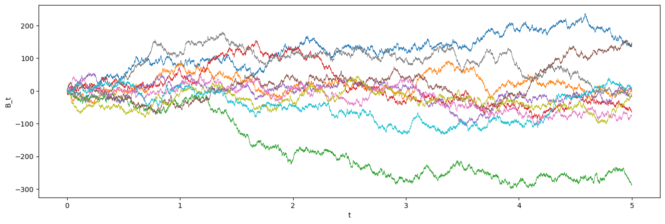
- Brownian motion: Think of a dust particle wiggling randomly in water. This is the basic “randomness” the models add.
- Itô calculus: Rules for handling equations that include random wiggles (like a “calculus for noise”).
- Adding noise and reversing it:
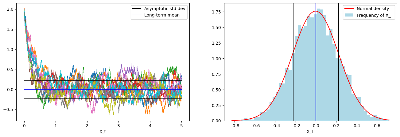
- Ornstein–Uhlenbeck process: Imagine a ball attached to a spring at the origin that’s constantly jiggled by random hits. Over time, anything you throw in gets pulled toward the center while being noised. This is a classic way to “destroy” information in data in a controlled way.
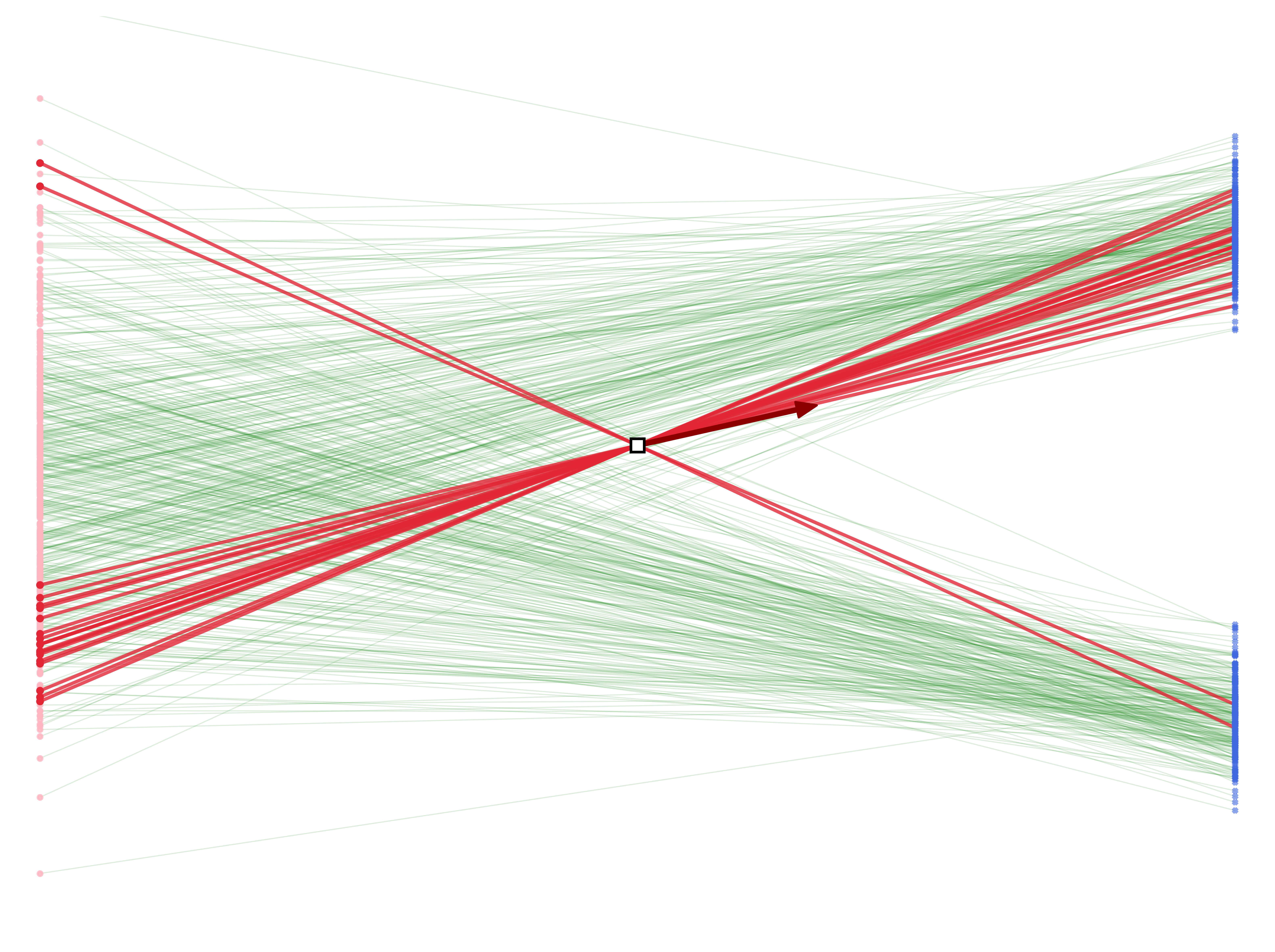
- Fokker–Planck equation: Picture a fog of points (a probability cloud). This equation tells how that fog spreads and moves over time when you add noise and drift.
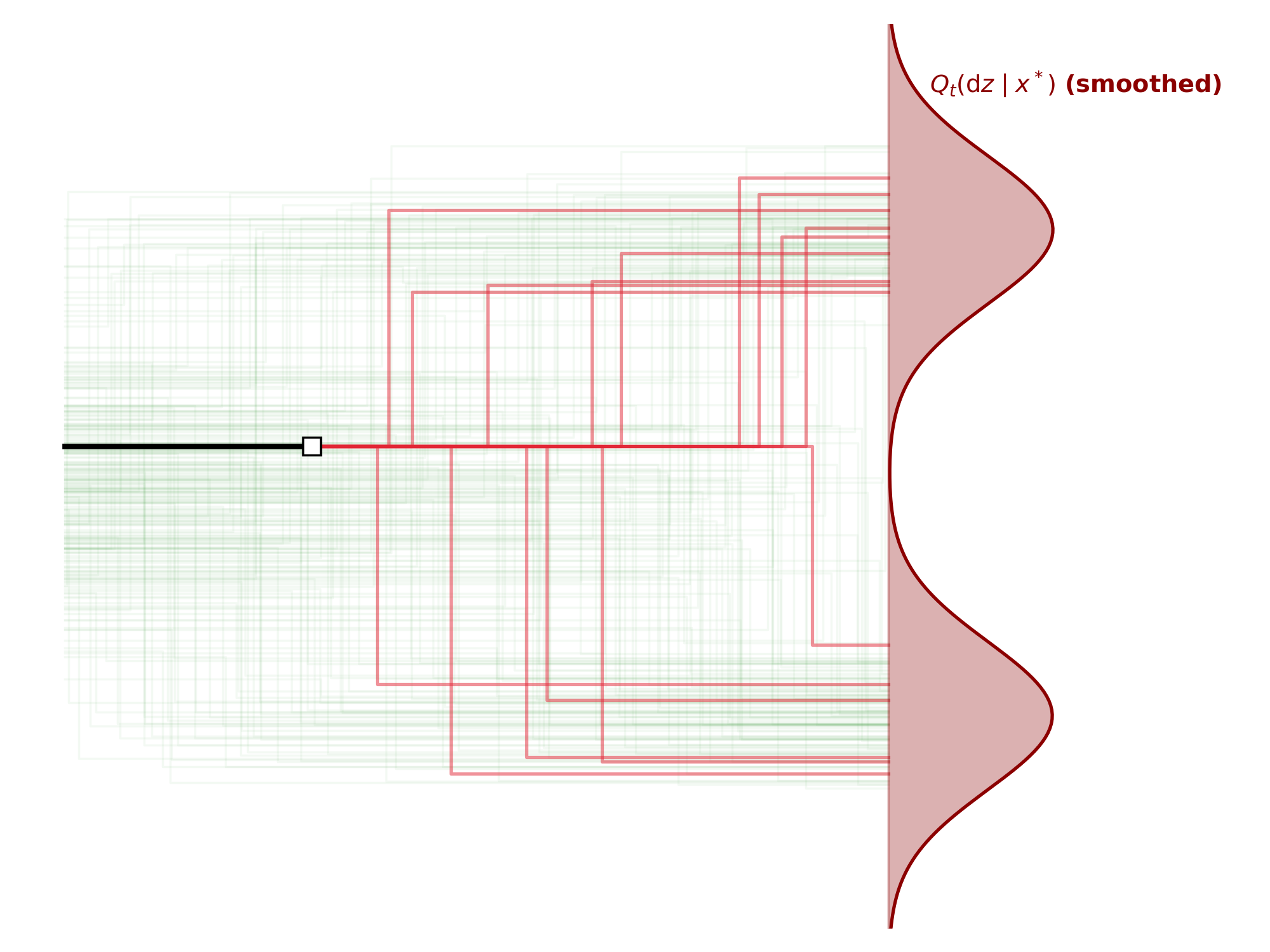
- Time reversal: If you understand how the fog changes forward in time, you can write the exact rules to run it backward—from pure noise back to structured data. The paper shows how to do this precisely.
- A cleaner, forward-time view:
- Instead of thinking “run time backward,” they re-label time so everything runs from (pure noise) to (data). This makes algorithms easier and less error-prone.
- Building paths from noise to data:
- Flow matching: Choose a simple path that moves a point from noise to a data sample (imagine drawing a straight line from a random point to a real example). Then learn a “velocity field” (a wind) that moves the entire fog along that path. This can be done by training a neural network using ordinary regression (predicting where to move).
- Gaussian paths: Another option is to make the in-between steps Gaussian (like blurring toward the target), which makes many formulas simple and sampling easy.
- Learning the “score” (the compass to high-density areas):
- The score is , which points in the direction where data is more likely. If you know the score, you can steer noise toward data.
- Score matching (vanilla): A math trick turns “match the true score” into a loss you can compute from samples, but it needs computing divergences (costly in high dimensions).
- Denoising score matching: A clever shortcut. Add known Gaussian noise to data, then train a network to predict that noise from the noised input. Surprisingly, doing this teaches the network the score—no expensive derivatives needed. This is why diffusion models train by “predicting noise.”
- Measuring how good generation is:
- KL divergence (think: a number that says how different two fogs are). The notes derive formulas that connect the final error of your generator to:
- how far your learned score is from the true score along the path, and
- how well your starting noise matches the theoretical ending of the forward noising process.
Main findings and why they matter
- A unified framework: The notes show that diffusion models, score-based models, and flow matching can all be expressed in one forward-in-time setup on . This removes the need to juggle backward time in code.
- Exact reverse rules: They derive the exact backward stochastic rules (how to go from noise to data) from the forward noising rules, guaranteeing that, in theory, you can perfectly reverse the process if you know the score.
- Practical training recipes:
- For flow matching: learn a velocity field by straightforward regression on simple synthetic pairs (noise + data).
- For score-based models: use denoising score matching—train a network to predict the noise you added. This gives you the score you need for generation.
- Quality guarantees: They prove bounds showing that if your learned score is accurate and your starting noise is set correctly, your generated samples will be close to the real data distribution. This gives a clear target for improving models: better score estimates → better samples.
What this means going forward
- Clearer design of generative models: With a single, math-consistent view, it’s easier to design, combine, and compare different methods (flows, diffusions, and hybrids).
- Easier, stable training: The denoising trick explains why predicting noise works so well in practice and avoids expensive computations.
- Better reliability: The error bounds help researchers understand and control where generation might go wrong, guiding better training schedules and architectures.
- New possibilities: By seeing flows and diffusions as two sides of the same coin, researchers can invent new samplers and training strategies that borrow the best of both worlds.
In short, the notes turn the idea “add noise to data, then learn to reverse it” into a clean, unified, and provably sound toolbox—making generative models both practical and trustworthy.
Knowledge Gaps
Knowledge gaps, limitations, and open questions
Below is a consolidated list of concrete gaps and open problems that remain unresolved in the paper, structured to guide future research.
Theoretical foundations and assumptions
- Clarify minimal regularity assumptions for all PDE/SDE manipulations: precise conditions on densities (existence, smoothness, positivity), boundary behavior (vanishing at infinity), and filtrations under which integration by parts, Fokker–Planck derivations, and time-reversal arguments are valid.
- Specify existence/uniqueness conditions for SDE/ODEs with learned (neural) drifts and state-dependent diffusion, including Lipschitz, growth, and measurability assumptions needed to guarantee well-posedness.
- Make the probability-flow ODE equivalence precise: state conditions ensuring that the ODE with velocity field exactly matches SDE marginals (e.g., absolute continuity, invertibility of flows, non-degenerate diffusion).
- Provide a rigorous statement of Anderson’s time-reversal theorem in the general, potentially state-dependent diffusion setting used here (beyond diagonal/scalar cases), including required smoothness of and non-degeneracy of the diffusion matrix.
- Analyze heavy-tailed or non-vanishing boundary mass cases where integration-by-parts steps and the “vanish at infinity” assumption fail; propose alternative formulations or weighted score objectives for such distributions.
Training objectives and statistical guarantees
- Connect the denoising score matching (DSM) training objective to the final-time KL bound: derive non-asymptotic generalization guarantees that translate empirical DSM error (with time-weighting ) into the integral score-error term in Proposition “KL bound for diffusion models.”
- Determine optimal time-weighting for DSM that minimizes the KL bound (which weights errors by ); provide a principled choice of aligned with the theoretical weight.
- Quantify how finite-sample error, model misspecification, and optimization error in learning compound along the generative trajectory to affect .
- Establish sample complexity and dimension-dependent rates for learning via DSM/flow matching under smoothness/Lipschitz assumptions on the ground-truth score (only hinted by cited future work).
- Analyze identifiability and non-uniqueness of feasible velocity fields in flow matching: characterize when multiple yield the same continuity equation and how this impacts learning with finite-capacity neural networks.
Schedules, noise design, and path choices
- Optimize the backward noise schedule : since the KL bound scales with , determine per-time optimal given expected score error profiles. (Note: the factor is minimized by , but the paper does not analyze how this interacts with training or data.)
- Study the selection of and base distribution to control the mismatch term and derive a principled trade-off between forward-noising duration and base mismatch.
- Characterize admissible families for Gaussian interpolating paths ensuring ; provide conditions and constructive schedules ensuring nonnegativity and stability as .
- Compare interpolation families (linear, OU-based, nonlinear ) theoretically: how do choices of and affect learnability of the score and the induced error weight in the KL bound?
State-dependent diffusion and beyond-Gaussian settings
- Extend the derivations to general, state-dependent diffusion matrices (not just scalar/diagonal): provide time-reversal formulas, transport velocities, and DSM targets for anisotropic noise.
- Develop DSM and flow matching for non-Gaussian conditional paths and noise distributions (beyond isotropic Gaussian), including explicit score targets and stability analysis.
- Explore extensions to manifold-valued data and constrained domains where Euclidean gradients/log-densities and boundary conditions require geometric or reflecting-boundary treatments.
Discretization, numerical stability, and implementation
- Quantify discretization error: provide strong/weak error bounds for discretized SDE/ODE solvers and translate them into deviations in final-time KL or Wasserstein distances.
- Analyze the regime where and DSM targets blow up; specify reweighting or schedule designs to avoid numerical instability near terminal time.
- Compare robustness of probability flow ODE vs. reverse SDE under approximate scores: which is more stable to systematic score bias or variance at different ? Provide error-to-divergence transfer bounds for both choices.
- Provide conditions under which neural drifts guarantee stable numerical integration (e.g., spectral norms/Lipschitz constraints) and quantify how such constraints affect approximation error.
Modalities and data types
- Address discrete or hybrid data (e.g., categorical, text) within this continuous-time framework: how to adapt DSM/flow matching and time-reversal when densities do not exist in the classical sense.
- Investigate behavior with multimodal, heavy-tailed, or low-dimensional manifold-supported : how do these characteristics affect the estimability of the score and the validity of PDE/SDE assumptions?
Tightness and refinement of the KL bound
- Assess the tightness of the KL bound that relies on Young’s inequality; explore refined inequalities or problem-specific coercivity (e.g., log-Sobolev, Poincaré) to obtain sharper constants or alternative control metrics (e.g., , Wasserstein).
- Develop lower bounds or converse results to understand when small DSM error is necessary for small final-time KL and whether there exist regimes where the current bound is vacuous (e.g., causing blow-ups).
Likelihoods, evaluation, and calibration
- Connect the framework to likelihood estimation: derive tractable estimators or bounds on or bits-per-dimension using the learned score/drift and discretized solvers.
- Provide guidance on calibrating score magnitudes across (e.g., via Tweedie’s formula) for consistent denoising and unbiased sampling, especially near endpoints where variances are extreme.
These directions aim to turn the paper’s elegant continuous-time view and foundational derivations into rigorous, practically reliable, and broadly applicable methodologies.
Practical Applications
Practical Applications of “Statistical Analysis of Markovian Generative Modeling”
This mini-course synthesizes a unified, forward-time framework for score-based diffusion models and flow matching, including (i) explicit kinematic and Gaussian interpolating paths from noise to data, (ii) regression-based training objectives for drifts and scores (flow matching and denoising score matching), (iii) probability-flow ODE/SDE samplers, and (iv) KL-based tracking of distributional mismatch. Below are actionable applications derived from these methods.
Immediate Applications
These can be deployed with current tools (e.g., PyTorch/JAX, torchsde/diffrax, existing diffusion/flow codebases).
- Software/Media: Simplified training pipelines for diffusion and flow models
- Use case: Implement forward-time training with Gaussian interpolants and denoising score matching (DSM), avoiding backward-time PDEs and costly divergence terms.
- Workflow/products:
- Training: sample data x₁∼p*, noise ξ∼N(0, I), time t∼U[0,1]; construct X_t = m_t(x₁)+σt ξ; train score sθ(X_t, t) via DSM or drift/velocity via (conditional) flow matching.
- Inference: choose SDE/ODE sampler; integrate from p₀≈N(0, I) (or matched OU base) to t=1.
- Offer as SDK components: “interpolant builder,” “drift/score trainer,” “SDE/ODE samplers.”
- Assumptions/dependencies: Adequate compute and network capacity; choice of schedules (α_t, σ_t, b_t) and solver tolerances; i.i.d. data; densities sufficiently regular (used in derivations).
- Software/Embedded: Deterministic, reproducible generation via probability-flow ODEs
- Use case: On-device or latency-sensitive applications (image/audio synthesis, denoising, inpainting) where stochasticity and sampling variance are undesirable.
- Workflow/products: Export trained score into a probability-flow ODE; integrate with fixed-step or adaptive solvers for deterministic outputs; provide quality/speed trade-off presets.
- Assumptions/dependencies: ODE integration accuracy; speed-quality tuning; trained score quality.
- Healthcare: Data augmentation and denoising for medical imaging and signals
- Use case: Improve classifier/segmenter generalization with synthetic MR/CT images or ECG waveforms generated via forward-time diffusion/flow pipelines; apply score models for denoising.
- Workflow/products: Fine-tune generic pipelines on domain data; use DSM for stable training; deploy ODE sampler for deterministic augmentation; integrate uncertainty via SDE for ensembles.
- Assumptions/dependencies: Ethical/data-use constraints; domain shift monitoring; clinical validation; careful control of artifacts.
- Finance/Energy: Scenario generation and stress testing
- Use case: Generate plausible future scenarios for risk, load, or price trajectories using learned stochastic generative SDEs; sample ensembles for uncertainty quantification.
- Workflow/products: Train interpolant-based models on historical time series; generate path ensembles; integrate with downstream risk/optimization tooling.
- Assumptions/dependencies: Stationarity or explicit conditioning; drift/volatility schedules adapted to time series; governance and audit of synthetic outputs.
- Robotics/Autonomy: Stochastic trajectory priors and planning
- Use case: Use generative SDEs to sample feasible trajectories or states from prior distributions; switch to ODE for reproducible rollouts.
- Workflow/products: Train on trajectory datasets using conditional flow matching (velocity regression targets); use forward SDE during exploration and ODE at deployment.
- Assumptions/dependencies: State/action representation compatibility; solver stability in high-dimensional control spaces.
- Privacy-preserving synthetic data (Industry/Policy)
- Use case: Train forward-time models to produce synthetic tabular or imaging data for sharing and benchmarking while reducing direct disclosure risk.
- Workflow/products: DSM training with calibrated noise schedules; integrate membership inference and privacy audits; provide data-card documentation.
- Assumptions/dependencies: Privacy is not guaranteed by default; evaluate re-identification risks; domain expertise for safe use.
- Research/Education: Reproducible teaching and benchmarking kits
- Use case: Curricula and labs demonstrating Brownian/OU processes, Fokker–Planck-to-transport connections, score matching, and flow matching with code templates.
- Workflow/products: Notebooks implementing OU, DSM, flow matching regressions, and SDE/ODE sampling; visualizations of continuity equations and velocity fields.
- Assumptions/dependencies: Standard scientific Python/JAX stacks; didactic datasets.
- Model diagnostics: Training and sampling guidance via KL transport calculus
- Use case: Use the KL time-derivative identity to design diagnostics that relate drift mismatch to divergence growth; guide schedule and solver choices.
- Workflow/products: Approximate the integrand (e.g., via trajectory-weighted quantities) to produce training-time indicators tied to score error and b_t choice; use as early-stopping or scheduler tuning signals.
- Assumptions/dependencies: The exact bound uses expectations under true p_t and true score (not available); use approximations/estimates as heuristics.
Long-Term Applications
These require additional research, scaling, or domain-specific adaptation before broad deployment.
- Regulated AI assurance: Quantitative guarantees for generative outputs (Healthcare/Finance/Gov)
- Use case: Leverage the KL-bound result connecting final divergence to score error and schedule choice to develop certification protocols.
- Potential products: Auditing toolkits estimating surrogate upper bounds; standardized test batteries and reporting for generative compliance.
- Dependencies/assumptions: Practical, computable surrogates for intractable expectations; validated estimators of score error; domain-specific risk thresholds.
- Physics-informed generative solvers and inverse problems (Science/Engineering)
- Use case: Couple the Fokker–Planck-as-transport formulation with physical constraints or priors to solve PDE-constrained sampling/inversion (e.g., geophysics, materials).
- Potential products: Hybrid solvers that blend deterministic probability-flow ODEs with constraint projections; stochastic interpolant flows tailored to physics.
- Dependencies/assumptions: Accurate physical models/constraints; numerical stability in large-scale PDEs; bespoke schedules and architectures.
- Adaptive/control-theoretic samplers
- Use case: Interpret schedule b_t and drift shaping as control inputs; design adaptive controllers for faster, more stable sampling with quality guarantees.
- Potential products: Closed-loop controllers that adjust step sizes and diffusion strength online; optimal-control-inspired policies for sampler efficiency.
- Dependencies/assumptions: Real-time estimation of local score error; robust control design; theoretical analysis of stability/optimality.
- Hybrid flow–diffusion systems for efficient likelihoods (Software/ML)
- Use case: Combine normalizing flows with stochastic interpolants (as the notes connect) for models with both fast inference and tractable likelihoods.
- Potential products: Libraries for “flow-with-noise” architectures enabling NLL evaluation and fast sampling; compression-friendly generative codecs.
- Dependencies/assumptions: Architecture engineering for high-dimensional data; training stability; calibration of likelihoods.
- Large-scale, domain-specific conditional generation
- Use case: Extend conditional Gaussian paths and conditional flow matching to strongly-conditioned tasks (e.g., multi-modal medical imaging, conditional weather nowcasting).
- Potential products: Foundation models for conditional generative tasks with domain adapters; APIs for plug-in conditions (text, tabular covariates, physical fields).
- Dependencies/assumptions: High-quality paired data; scalable conditioning mechanisms; domain validation and interpretability.
- Formal privacy and fairness frameworks for generative synthetic data
- Use case: Integrate denoising/flow matching with differential privacy mechanisms and fairness constraints; leverage transport identities to track distribution shifts.
- Potential products: DP-aware training for generative SDEs/ODEs; fairness diagnostics based on transport metrics; policy toolkits for safe data release.
- Dependencies/assumptions: Utility–privacy–fairness trade-off studies; legal/regulatory alignment; robust metrics.
- Edge-native generative inference
- Use case: Optimize probability-flow ODEs for edge devices (phones, IoT) for personalized but private content synthesis.
- Potential products: Quantized ODE samplers; schedule-aware distillation (few-step ODEs); on-device pipelines for personalization.
- Dependencies/assumptions: Model compression/distillation research; hardware constraints; energy-aware solvers.
- Theoretical-to-practical bridges: generalization and Lipschitz regularity
- Use case: Operationalize cited generalization/Lipschitz results into training-time regularizers that guarantee sampling rates and stability.
- Potential products: Regularization plugins enforcing Lipschitz constraints on score/drift; adaptive weighting tied to proven rates.
- Dependencies/assumptions: Translating bounds to practical estimators; impact on sample quality and diversity.
Cross-cutting assumptions and dependencies
- Mathematical assumptions used in the notes (e.g., smooth densities, decay at infinity, existence/uniqueness of SDE solutions) are approximated in practice; deviations can affect guarantees.
- Quality depends on score/drift network capacity, data coverage, and the choice of time/noise schedules (α_t, σ_t, b_t).
- Numerical stability hinges on ODE/SDE solver choices (stepsize, tolerances) and stiffness of learned dynamics.
- For sensitive domains (healthcare, finance), external validation, governance, and safety monitoring are necessary; theoretical identities should be treated as guides unless computably instantiated.
Glossary
- Anderson's theorem: A result in stochastic processes that underpins time-reversal of diffusions and the construction of backward SDEs from forward ones. "one can reinterpret the Fokker-Planck equation to explicitly derive the backward SDE mapping noise back to data (a consequence of Anderson's theorem)."
- Brownian motion: A continuous-time stochastic process with independent Gaussian increments, serving as the fundamental noise process in stochastic calculus. "There exists a process called Brownian motion, which is a centered Gaussian process over "
- Brownian scaling: The scaling property of Brownian motion that relates time-rescaled Brownian paths to a standard Brownian motion. "Brownian scaling "
- Continuity equation: A PDE expressing conservation of probability mass under a velocity field, often written as . "if we assume that satisfies a continuity equation "
- Covariance kernel: A function giving the covariance between values of a stochastic process at times and . "The distribution of a centered Gaussian process is fully determined by its covariance kernel "
- Denoising Diffusion Probabilistic Models (DDPM): A class of generative models that learn to reverse a noising diffusion process to synthesize data. "Application to Denoising Diffusion Probabilistic Models (DDPM)"
- Denoising score matching: A technique to estimate the score (gradient of log-density) of a noisy distribution by regressing against the known noise score, avoiding computing divergences of the model. "As will be rigorously proven in Section~\ref{sec:denoisingscorematching} through Denoising Score Matching, we can bypass the intractable marginal score ."
- Donsker's invariance principle: A functional central limit theorem linking scaled random walks to Brownian motion. "A geometric construction on uses Donsker's invariance principle."
- Drift (of an SDE): The deterministic component of an Itô stochastic differential equation, often denoted in . "Here is the drift and the diffusion term (or volatility)."
- Filtration: An increasing family of σ-fields representing the accumulation of information over time. "A filtration over is an increasing family $(F_t)_{t \in \mathcal{T}$ of -fields, i.e.\ for all ."
- Fisher divergence: A discrepancy measure between probability distributions based on the difference of their score functions. "The fundamental metric is the Fisher divergence:"
- Fokker-Planck equation: A PDE that governs the time evolution of the probability density of a diffusion process. "Then has a density satisfying the Fokker-Planck equation:"
- Gaussian process: A stochastic process where any finite collection of points has a joint Gaussian distribution. "A (real-valued) random process is called a (centered) Gaussian process if any finite linear combination of the variables $(X_t)_{t \in \mathcal{T}$ is a centered Gaussian."
- Hölder continuity: A regularity condition describing functions whose increments are bounded by a power of the distance, here with exponent less than 1/2 for Brownian paths. "they are locally Hölder continuous with exponent for all ."
- Itô formula: A stochastic chain rule that extends the classical chain rule to Itô processes. "Multidimensional Itô formula"
- Itô integral: An integral with respect to Brownian motion defined via mean-square limits, central to stochastic calculus. "However, we can construct the Itô integral using the finiteness of its quadratic variation."
- Itô isometry: An identity stating that the second moment of an Itô integral equals the integral of the integrand’s second moment. "This yields the crucial Itô isometry: ."
- Itô process: A process that can be decomposed into a drift term and a diffusion term driven by Brownian motion. "An Itô process is a stochastic process adapted to which can be written as"
- Kolmogorov’s continuity criterion: A result ensuring the existence of continuous versions of stochastic processes under moment conditions. "From Kolmogorovâs continuity criterion, they are locally Hölder continuous with exponent "
- Kullback–Leibler divergence: An information-theoretic measure of discrepancy between two probability distributions. "The following result allows us to track the KL divergence between two probability flows driven by generic transport equations."
- Laplacian: A second-order differential operator ; in Fokker–Planck, it models diffusion. "The FokkerâPlanck equation can be recast as describing the pure transport of mass corresponding to a deterministic ODE by factoring the Laplacian term."
- Martingale: A stochastic process with constant conditional expectation given the past, capturing “fair game” dynamics. "the Brownian motion is a martingale adapted to the filtration "
- Ornstein–Uhlenbeck process: A mean-reverting Gaussian diffusion often used as a forward noising process in diffusion models. "An Ornstein-Uhlenbeck (OU) process with parameters starting at is defined by:"
- Quadratic variation: The limit of the sum of squared increments of a process; for Brownian motion it equals elapsed time. "its quadratic variation is always well defined and deterministic."
- Score function: The gradient of the log-density, , used to define probability flow dynamics in score-based models. "The only unknown term required to run the simulation is the score function ."
- Score matching: A method to estimate the score function by minimizing discrepancies that avoid normalizing constants. "The main trick for score matching dates back to~\cite{hyvarinen2005estimation}."
- Score-based generative models (SGM): Generative methods that learn and follow the score of intermediate noised distributions to sample data. "Recovering Score-based generative models (SGM)"
- Stochastic differential equation (SDE): An equation involving differentials driven by stochastic processes like Brownian motion. "we obtain the explicit backward generative SDE:"
- Stochastic time-reversal: The reversal of a stochastic process in time to construct backward dynamics consistent with forward marginals. "Stochastic time-reversal (Anderson's theorem)"
- Transport equation: A PDE of the form modeling the flow of density under a velocity field. "can be recast as the non-linear transport equation:"
- Tweedie’s formula: A relation connecting the posterior mean under Gaussian noise to the score of the marginal, used to interpret score learning as denoising. "Tweedie's formula: learning the noise"
- Velocity field: A vector field that transports probability mass in deterministic or stochastic generative flows. "we see that one valid velocity field is exactly the conditional expectation:"
- Young’s inequality: An inequality bounding inner products by weighted sums of norms, used to control terms in analysis. "where the inequality follows from Young's inequality"
- σ-field (sigma-field): A collection of sets closed under complements and countable unions, encoding events measurable at a given time. "the -field "
Collections
Sign up for free to add this paper to one or more collections.