Equilibrium Matching: Generative Modeling with Implicit Energy-Based Models
Abstract: We introduce Equilibrium Matching (EqM), a generative modeling framework built from an equilibrium dynamics perspective. EqM discards the non-equilibrium, time-conditional dynamics in traditional diffusion and flow-based generative models and instead learns the equilibrium gradient of an implicit energy landscape. Through this approach, we can adopt an optimization-based sampling process at inference time, where samples are obtained by gradient descent on the learned landscape with adjustable step sizes, adaptive optimizers, and adaptive compute. EqM surpasses the generation performance of diffusion/flow models empirically, achieving an FID of 1.90 on ImageNet 256$\times$256. EqM is also theoretically justified to learn and sample from the data manifold. Beyond generation, EqM is a flexible framework that naturally handles tasks including partially noised image denoising, OOD detection, and image composition. By replacing time-conditional velocities with a unified equilibrium landscape, EqM offers a tighter bridge between flow and energy-based models and a simple route to optimization-driven inference.


Paper Prompts
Sign up for free to create and run prompts on this paper using GPT-5.
Top Community Prompts
Explain it Like I'm 14
Overview: What this paper is about
This paper introduces a new way to make AI generate images, called Equilibrium Matching (EqM). Instead of using a time-based process like many popular methods (diffusion or flow models), EqM learns a single, steady “force field” that pulls noisy images toward clear, realistic ones. You can think of it like shaping a landscape of hills and valleys where real images sit at the bottom (valleys). To generate a picture, EqM drops a point on this landscape and lets it “roll downhill” into a realistic image.
The big idea: learn one stable landscape (an energy landscape) and then use simple optimization (like gradient descent) to sample images. This makes sampling flexible, fast, and high-quality—EqM achieves top results on a big benchmark (ImageNet 256×256) with an FID of 1.90, where lower is better.
Key objectives and questions
- Can we replace time-dependent, step-by-step denoising (used by diffusion/flow models) with a single, time-free “equilibrium” force field that always points from noise toward real images?
- How do we design targets during training so the learned force field naturally comes from an underlying energy landscape (with real images at the “valleys”)?
- Can we sample by simple optimization (like gradient descent), using flexible step sizes, better optimizers (like Nesterov momentum), and even stop early when we’re close enough?
- Will this approach beat or match state-of-the-art image generation quality?
- Does it unlock useful abilities, like denoising partially corrupted images, detecting out-of-distribution (unfamiliar) inputs, or composing images by combining models?
How EqM works (in everyday terms)
Imagine a landscape:
- Valleys = real images
- Hills = noise
- Arrows = directions showing how to move from any point toward a valley
EqM learns these arrows (the gradient) so that:
- The arrows are strong in noisy areas (pushing you toward real images),
- They fade to zero as you arrive at the real image (so you stop in the valley),
- And they don’t depend on a time step—there’s just one, steady landscape.
Here’s how they train it:
- Mix a real image x with pure noise ε using a blend factor γ (like a slider from 0 to 1):
- If γ=0: you have pure noise
- If γ=1: you have the clean image
- In between: a partially noised image x_γ
- Teach the model to predict an arrow that points from noise toward the real image, and to make that arrow smaller as γ gets closer to 1 (i.e., near real images the arrow should be near zero). This “shrinking” is controlled by a function c(γ) with c(1)=0.
Why this matters: If the arrows vanish at real images, then those points are stable resting places (valleys). That’s exactly what an energy landscape should look like.
Two flavors of EqM:
- Implicit energy: learn the arrows directly (the gradient), without explicitly storing the “height” (energy) of the landscape.
- Explicit energy (EqM-E): also learn an energy value for each point, so you can rank how “in-distribution” something is (useful for detecting unusual inputs). They describe simple ways to get this energy from the model’s outputs.
Sampling (how EqM generates images):
- Start from random noise (a point on the hills),
- Repeatedly move a small step in the direction the arrows suggest (gradient descent),
- Optionally use better “rolling” strategies like Nesterov Accelerated Gradient (a look-ahead trick),
- Choose any step size you like, and even stop early when the arrows get tiny (meaning you’re near a valley).
Compared to diffusion/flow methods that follow a fixed, time-conditioned path, EqM’s optimization view is more flexible: step sizes, optimizers, and number of steps are all adjustable.
Main results and why they matter
Highlights:
- Stronger image quality: On ImageNet 256×256 (class-conditional), EqM reaches FID 1.90, outperforming strong diffusion/flow baselines (lower FID is better image quality).
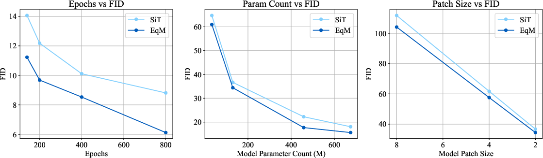
- Scales well: As the model size, training time, or image patch settings increase, EqM consistently beats comparable flow models.
- Flexible, optimization-style sampling:
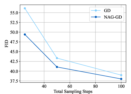
- Works with simple gradient descent or with Nesterov momentum for better quality, especially with fewer steps.
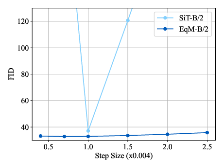
- Robust to step size choices (unlike many flow samplers that need a very specific step).
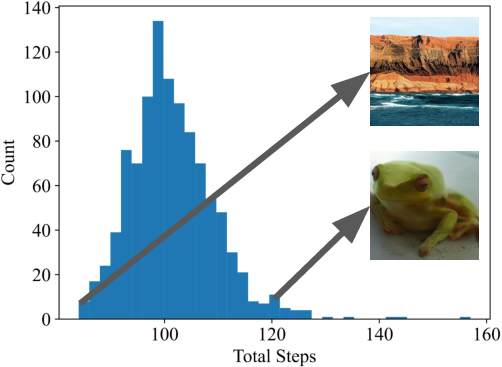
- Adaptive compute: can stop early per image when the gradient gets small, saving up to about 60% of function evaluations in tests.
- New abilities:
- Partially noised input denoising: If the input is only a little noisy, EqM naturally produces better results, without needing a special “noise level” input. Flow/diffusion models often struggle here unless you tell them the exact noise level.
- Out-of-distribution detection: With explicit energy, unusual images tend to have higher energy. EqM shows strong average performance compared to popular baselines.
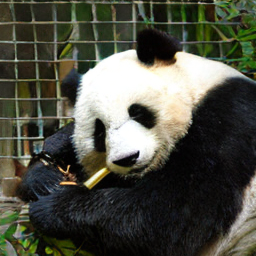
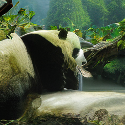
- Composition: You can add two EqM models (e.g., “panda” and “valley”) by adding their energies/gradients to generate combined images. This is simple and mirrors classic energy-based model compositionality.
Theory (intuitive takeaways):
- Real images have near-zero gradient (no arrows), so they’re local minima (valleys).
- The local minima the model learns are very likely to be real data points.
- Gradient-descent sampling provably makes progress under standard smoothness assumptions, with a convergence rate that improves as you take more steps.
Implications and potential impact
EqM bridges two worlds:
- The practicality and high quality of flow/diffusion methods,
- The interpretability and flexibility of energy-based models.
Because sampling is “just optimization,” EqM:
- Makes it easy to tune speed/quality trade-offs (change step size, number of steps, optimizer),
- Can adapt compute per sample,
- Naturally supports tasks like denoising partial noise, anomaly detection, and combining concepts.
In short, EqM offers a simpler, more flexible route to high-quality generation with promising new abilities that could help in areas like image editing, safety (detecting unusual inputs), and creative composition.
Knowledge Gaps
Knowledge gaps, limitations, and open questions
Below is a single, actionable list of what remains missing, uncertain, or unexplored in the paper that future work could address:
- Integrability of the learned vector field: EqM trains an implicit gradient f(x) without enforcing curl-free constraints, so it is unclear when f is conservative and truly corresponds to ∇E; measuring and regularizing the non-conservative (rotational) component is an open need.
- Explicit energy training degradation: EqM-E variants hurt generation quality and can be unstable (especially the L2 norm variant); it is unclear how to stabilize explicit-energy training or co-train scalar energy and vector field without sacrificing sample quality.
- Theoretical assumptions vs practice: Guarantees hinge on perfect training, high-dimensional approximations, and L-smoothness; practical, finite-sample bounds (with model misspecification and optimization error) on convergence, spurious minima, and generalization remain unproven.
- Data-distribution fidelity: The theory ensures vanishing gradients at data points but does not show that the stationary distribution (or sample distribution) matches the true data distribution; likelihood connections or consistency guarantees are missing.
- Objective design c(γ): The choice of c(γ) is heuristic; a principled derivation (e.g., from maximum-likelihood, score matching, or contrastive objectives) and dataset-agnostic selection/learning of c(γ) are open questions.
- Corruption scheme generality: Only linear interpolation with Gaussian noise is studied; the impact of non-Gaussian/noise types, more realistic corruptions, or data-dependent corruptions on training stability and quality is unknown.
- Hyperparameter robustness: Performance depends on a and λ; sensitivity analyses across datasets/scales and automatic tuning strategies (e.g., adaptive λ or learned c(γ)) are not provided.
- Sampling stability and step-size control: Robustness is shown empirically for a range of fixed η, but there is no analysis or implementation of adaptive step-size control (e.g., backtracking line search, Lipschitz estimation) and its effects on quality/speed.
- Optimizer space for sampling: Only GD and NAG are evaluated; how momentum schedules, Adam/RMSProp/Adagrad/L-BFGS, adaptive restarts, or second-order updates affect quality, speed, and stability is unexplored.
- Adaptive compute stopping criteria: Stopping by ||∇E|| < g_min lacks calibration analysis; the trade-off between early stopping, sample bias, quality variance, and compute savings across datasets and models remains uncharacterized.
- Diversity and mode coverage: Evaluation relies on FID; precision/recall, density-and-coverage, and other diversity/coverage metrics (and failure cases such as mode dropping) are not reported.
- Likelihood/NLL estimation: No bits-per-dim or NLL is reported; it is unknown whether EqM can be related to tractable likelihood surrogates or whether it admits practical likelihood estimation schemes.
- Fairness of compute comparisons: The paper does not provide matched wall-clock, FLOPs, or GPU-day comparisons to diffusion/flow baselines (training and sampling), leaving unclear whether EqM’s quality gains come with higher compute.
- Scaling breadth: Results focus on ImageNet 256×256; behavior at higher resolutions (512/1024), small images (e.g., CIFAR-10), other modalities (audio, video), and different architectures (e.g., U-Nets) is untested.
- Conditioning mechanisms and guidance: Details of class conditioning (e.g., classifier-free guidance usage/strength) are under-specified; how to design guidance analogs in EqM (and trade off fidelity vs realism) is an open design space.
- Partial-noise denoising fairness: The comparison to FM on partially noised inputs may be unfair since FM expects explicit noise conditioning; evaluating EqM vs properly noise-aware FM baselines on restoration tasks (e.g., known-noise denoising, inpainting, super-resolution) is needed.
- OOD detection protocol clarity: The dataset used to train the EqM-E model for OOD detection, preprocessing, energy calibration/scaling, and statistical variability are not fully specified; broader benchmarks and ablations are needed.
- Composition correctness and limits: Gradient addition is demonstrated qualitatively, but quantitative evaluation, conflict analysis (when gradients disagree), weighting schemes, scaling to >2 conditions, and negative prompts remain open.
- Measuring and reducing non-conservative error: There is no diagnostic quantification (e.g., via Helmholtz decomposition) of the rotational component of f or ablations on penalties that enforce integrability; this could clarify why EqM-E underperforms.
- Initialization and training curricula: EqM-E (especially the L2 variant) requires careful initialization; whether pretraining schedules, curriculum on γ, or staged objectives improve stability or quality is unknown.
- Starting distribution and mixing: Sampling starts from Gaussian noise; the impact of alternative initializations (e.g., replay buffers, data-augmented starts), multi-start strategies for diversity, and mixing behavior across modes is not studied.
- Robustness and safety: Sensitivity to adversarial perturbations, spurious minima, dataset biases, and privacy risks (e.g., membership inference) in gradient-based samplers is unexamined.
- ODE/SDE connections: The claimed equivalence to ODE-based sampling is deferred to the appendix; a formal mapping of EqM’s optimization view to known ODE/SDE samplers (with/without diffusion terms) and when these coincide is not fully developed.
- Computational efficiency of EqM-E: Explicit-energy variants require Jacobian-related computations; practical strategies for efficient Jacobian-vector products or memory-saving techniques are not discussed.
- Multi-task trade-offs: Using explicit energy for OOD while keeping high generation quality appears difficult; joint training strategies that balance generation and downstream tasks (e.g., OOD, editing) are not explored.
Practical Applications
Practical Applications of Equilibrium Matching (EqM)
Below are the practical, real-world applications that emerge from the paper’s findings, methods, and innovations. Each item specifies sector(s), concrete use cases, potential tools/workflows, and assumptions or dependencies that may affect feasibility.
Immediate Applications
The following applications can be deployed now with EqM models trained on in-domain data (e.g., ImageNet) using the described training and sampling procedures.
- EqM-powered image generation pipelines
- Sectors: media/entertainment, advertising, e-commerce, gaming
- Use cases: high-fidelity image generation with improved FID; faster iterative creative workflows through optimization-based sampling (GD/NAG) and flexible step sizes; per-sample adaptive compute to reduce inference cost by up to ~60% function evaluations
- Tools/workflows: “EqM Sampler SDK” integrating NAG-GD or Euler ODE; inference servers with per-sample early stopping on gradient norm (g_min); sliders to adjust step size (η) and compute budget at runtime
- Assumptions/dependencies: availability of EqM models trained on the target domain; step-size and threshold tuning; adequate GPU/TPU resources; ImageNet results generalize to comparable image domains but require domain-specific fine-tuning
- Adaptive compute controllers for generative services
- Sectors: cloud/edge software, MLOps
- Use cases: budget-aware inference that auto-stops when gradients are small; dynamic SLA/latency management for content generation; cost reduction for batch generation
- Tools/workflows: middleware that monitors ||∇E(x)|| and applies early stopping; autoscaling policies that allocate compute based on real-time gradient statistics
- Assumptions/dependencies: calibration of g_min against quality metrics; monitoring for quality drift; robust fallback paths for samples that need more steps
- Partially noised image denoising without noise-level conditioning
- Sectors: consumer imaging, visual communications, scientific imaging, remote sensing
- Use cases: restoration/enhancement from partially corrupted inputs (low-light phone photos, surveillance frames, microscopy/astronomy sensor noise); unlike diffusion/flow, EqM improves as inputs get less noisy even without explicit noise-level inputs
- Tools/workflows: “NoisyImageFix” pipeline that feeds partially noisy images to EqM models directly; batch restoration services for archives and digitization projects
- Assumptions/dependencies: EqM must be trained/fine-tuned on representative data; performance may degrade under significant distribution shift or domain-specific artifacts (e.g., medical)
- Energy-based OOD detection for images
- Sectors: MLOps/data curation, security/content moderation, quality assurance
- Use cases: gatekeeping datasets, flagging anomalous or out-of-domain content before training; safety checks for generative pipelines (reject high-energy OOD inputs/outputs)
- Tools/workflows: “EnergyGate” plugin using dot-product EqM-E variant to compute energy per image; ROC/AUROC-based thresholding for OOD alarms
- Assumptions/dependencies: the explicit energy (EqM-E) dot-product variant is recommended (L2 variant is less stable and performs worse); thresholds must be calibrated; potential trade-off between best-in-class generation quality and explicit-energy training variants
- Compositional image generation by summing gradients
- Sectors: product design, education, creative tooling
- Use cases: blending multiple conditional concepts (e.g., “panda” + “valley”) via gradient addition; rapid ideation/prototyping of hybrid concepts
- Tools/workflows: “EqM Compose” UI that adds class-conditional gradients during sampling; extensible to multi-condition combinations with sliders for gradient weights
- Assumptions/dependencies: availability of class-conditional EqM models; careful weighting to avoid artifacts or domination by a single concept
- Robust sampling controls for on-demand quality/latency trade-offs
- Sectors: software tooling, interactive UIs
- Use cases: step-size (η) flexibility and optimizer choice (GD vs. NAG) to tune latency/quality on the fly; more robust than flow-based samplers that require a specific η
- Tools/workflows: inference interfaces exposing optimizer and step-size; per-session policies (e.g., NAG with μ≈0.3–0.35) for faster convergence at low step counts
- Assumptions/dependencies: EqM hyperparameters (e.g., truncated decay c(γ) with a≈0.8 and λ≈4) and sampler settings require modest tuning; extreme step sizes can still degrade quality
- Synthetic data generation for vision tasks
- Sectors: retail/e-commerce, automotive, industrial inspection
- Use cases: macro-scale image augmentation for training discriminative models; compositional synthesis to cover rare combinations; lower inference cost via adaptive compute
- Tools/workflows: “EqM Data Factory” with class-balanced sampling, compositional generators, and quality-check gates (EnergyGate)
- Assumptions/dependencies: domain shift considerations; downstream model fairness and bias audits; licensing/rights for generated assets
- Rapid research prototyping on equilibrium dynamics
- Sectors: academia/AI labs
- Use cases: systematic evaluation of optimization algorithms as samplers (e.g., NAG vs. Adam); analysis of learned energy landscapes (vanishing gradients at data manifold); benchmarking EqM vs. diffusion/flow on standard datasets
- Tools/workflows: open-source EqM training/sampling code; experiment suites varying c(γ), λ, optimizer, and step budgets
- Assumptions/dependencies: compute resources for training; reproducibility practices; careful experimental design for fair comparisons
Long-Term Applications
The following applications require further research, scaling, domain adaptation, or regulatory/operational development.
- Cross-modality EqM (audio, video, text, multimodal)
- Sectors: media, accessibility, communications
- Use cases: extend equilibrium dynamics and optimization-based sampling to non-image domains; unify EBMs and flows across modalities for efficient generation
- Tools/workflows: transformer backbones with modality-specific encoders; multi-condition gradient composition across text and image
- Assumptions/dependencies: architectural adaptations for sequence data; new training objectives and stability analyses; large-scale multimodal datasets
- Healthcare imaging (clinical denoising, OOD safety, data augmentation)
- Sectors: healthcare/medical imaging
- Use cases: denoising and restoration of MR/CT/X-ray scans; OOD detection for device shifts or rare pathologies; synthetic data augmentation under strict governance
- Tools/workflows: hospital PACS-integrated “EqM Restore” for low-dose scans; “EnergyGate” safety layer for distribution-shift detection in clinical workflows
- Assumptions/dependencies: rigorous validation on medical datasets; bias/safety analyses; regulatory approvals (FDA/CE); domain adaptation and calibration
- Robotics and autonomous systems (energy-guided scene synthesis and planning aids)
- Sectors: robotics, autonomous vehicles
- Use cases: compositional generation of complex scenes for simulation; energy landscape shaping to encode task constraints; potential gradient-guided sampling to find feasible states
- Tools/workflows: “EqM Sim Studio” to produce diverse training environments; composition of conditional energies (e.g., object + terrain + lighting)
- Assumptions/dependencies: transfer from image synthesis to 3D/physics-anchored domains; integration with control/planning stacks; safety validation
- On-device generative AI with energy-efficient inference
- Sectors: mobile/edge computing
- Use cases: latency- and power-aware generation via adaptive compute and step-size scheduling; selective early stopping for battery conservation
- Tools/workflows: hardware-aware sampling libraries using NAG and small GD steps; dynamic profiles based on device thermal/power states
- Assumptions/dependencies: lightweight EqM models or distillation; hardware optimizations (e.g., fused ops); careful user experience tuning
- Policy and standards for safety and efficiency in generative AI
- Sectors: public policy, industry governance
- Use cases: standardizing OOD detection practices (energy thresholds, AUROC reporting); compute/energy-efficiency reporting for generative systems; guidelines for compositional generation transparency
- Tools/workflows: audit templates for energy-based OOD; procurement standards favoring adaptive compute and equilibrium sampling
- Assumptions/dependencies: consensus-building and multi-stakeholder engagement; empirical benchmarks across domains; monitoring for misuse or unintended bias
- Fraud and anomaly detection beyond images (if EqM extends to structured/time-series data)
- Sectors: finance, cybersecurity, IoT/industrial
- Use cases: energy-based detection of anomalous sequences (transactions, logs, sensor streams)
- Tools/workflows: “EnergyGate” for sequence data; dashboards for risk triage based on energy distributions
- Assumptions/dependencies: successful adaptation of EqM to non-image modalities; demonstration of stability and AUROC gains vs. baselines; robust labeling and ground truth availability
- Interpretable model analysis via energy landscapes
- Sectors: AI safety, research, auditing
- Use cases: use vanishing-gradient property at manifold points to analyze model behavior; detect spurious minima or failure modes; inform training and sampler design
- Tools/workflows: visualization tools for ∇E(x), energy contours, and sampling trajectories; automated checks for landscape smoothness (L-smooth proxies)
- Assumptions/dependencies: reliable explicit-energy variants or proxy energies; scalability to large models/datasets; links between energy geometry and downstream reliability
Notes on key assumptions and dependencies across applications:
- Reported performance is on ImageNet 256×256 with transformer backbones; domain transfer requires fine-tuning and validation.
- Theoretical guarantees assume smooth energy and “perfect training” (idealized); practical systems must account for approximation and noise.
- Explicit-energy models enable OOD detection but may trade off generation quality and training stability; a dual-model approach (EqM for generation + EqM-E for energy scoring) may be pragmatic.
- Hyperparameters (e.g., truncated decay c(γ) with a≈0.8 and multiplier λ≈4; NAG μ≈0.3–0.35; step size η; g_min) need calibration per domain and deployment target.
Glossary
- Adaptive compute: Allocating per-sample inference steps/computation based on a stopping criterion rather than a fixed budget. "adjustable step sizes, adaptive optimizers, and adaptive compute."
- Adaptive optimizers: Optimization algorithms that adapt learning rates or moments during updates (e.g., Adam), here used during sampling. "adjustable step sizes, adaptive optimizers, and adaptive compute."
- AUROC: Area Under the Receiver Operating Characteristic; a threshold-independent metric for detection performance. "We report the area under the ROC curve (AUROC) in \cref{ood}."
- Class-conditional: Conditioning a generative model on class labels to control the output class. "We report performance on class-conditional ImageNet 256256 image generation."
- Composition: Combining multiple models or energy functions so their effects add, enabling compositional image generation. "Composition. EqM also naturally supports the composition of multiple models by adding energy landscapes together (corresponding to adding the gradients of each model)."
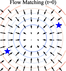
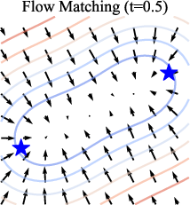
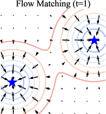
- Conditional velocity: A velocity field conditioned on input/time/noise level that defines the direction of the generative flow. "Flow Matching (FM), for example, learns to match the conditional velocity along a linear path connecting noise and image samples."
- Data manifold: The (typically lower-dimensional) set where true data lie, which models aim to learn and sample from. "EqM is also theoretically justified to learn and sample from the data manifold."
- Differential equation framework: Viewing sampling as integrating an ODE/SDE defined by the model’s predictions. "This process is governed by a differential equation framework, in which the predicted velocity is treated as the time derivative of the desired sampling path and integrated over a total length of $1$."
- Diffusion models: Generative models that learn to reverse a noising process to produce data from noise. "Diffusion models \citep{sohl,ddpm,ddim,nichol2021improved,dhariwal2021diffusion,edm} generate images from pure noise through a series of noising and denoising steps that are conditioned on noise level."
- Energy-based models (EBMs): Models that assign an energy to each input, with lower energy for data-like inputs, defining an unnormalized density. "Energy-based models (EBMs) \citep{hinton2002training,lecun2006tutorial, xie2016theory, du2019implicit, du2020improved, nijkamp2020anatomy, gao2020learning} learn an energy landscape that defines the unnormalized log-density of data distribution."
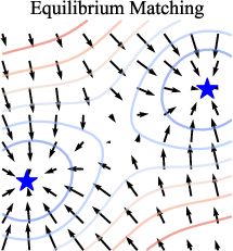
- Energy landscape: A scalar surface over inputs where data correspond to low-energy regions; its gradient guides sampling. "learns the equilibrium gradient of an implicit energy landscape."
- Equilibrium dynamics: Time-invariant dynamics characterized by gradients of a stationary energy function, as opposed to time-conditioned flows. "We introduce Equilibrium Matching (EqM), a generative modeling framework built from an equilibrium dynamics perspective."
- Equilibrium gradient: The gradient of an energy landscape that does not depend on time/noise; used for optimization-based sampling. "learns the equilibrium gradient of an implicit energy landscape."
- Equilibrium Matching (EqM): The proposed framework that learns a time-invariant gradient/energy function for generative modeling. "We introduce Equilibrium Matching (EqM), a generative modeling framework built from an equilibrium dynamics perspective."
- Equilibrium Matching with Explicit Energy (EqM-E): A variant that learns a scalar energy function whose gradient matches a target field. "The Equilibrium Matching with Explicit Energy (EqM-E) objective can be written as:"
- Euler (ODE) sampler: A first-order ODE integrator used to sample by stepping along predicted dynamics. "Euler {\scriptsize (ODE)}"
- FID: Fréchet Inception Distance; a standard metric measuring generative sample quality against real data. "achieving an FID of 1.90 on ImageNet 256256."
- Flow Matching (FM): A generative approach that learns velocities along interpolations between noise and data to define a flow. "Flow Matching (FM), for example, learns to match the conditional velocity along a linear path connecting noise and image samples."
- Gaussian noise: A normal distribution used as the noise source for initialization or corruption. "Flow Matching starts from pure Gaussian noise and iteratively denoises the current sample"
- Gradient descent (GD): An optimization method that iteratively updates inputs against the gradient to minimize energy. "Gradient Descent Sampling (GD)."
- Gradient multiplier: A scalar factor used to rescale the target gradient field during training. "we introduce an additional gradient multiplier on top of these gradient fields to control the overall scale."
- Gradient norm: The magnitude (often L2) of the gradient vector; used here as a convergence/early-stopping criterion. "stopping when the gradient norm drops below a certain threshold ."
- Heun (SDE): A numerical integrator (predictor-corrector) for stochastic differential equations used in sampling. "Heun {\scriptsize (SDE)}"
- Implicit Energy-Based Models: EBMs learned via their gradients without explicitly parameterizing the energy function. "Equilibrium Matching: Generative Modeling with Implicit Energy-Based Models"
- Implicit energy landscape: An energy function not explicitly parameterized, inferred via its learned gradient field. "learns the equilibrium gradient of an implicit energy landscape."
- Integration horizon: The total integration length/time over which dynamics are solved during sampling. "This non-equilibrium design imposes practical constraints such as noise level schedule and fixed integration horizon during sampling."
- Integration-based samplers: Samplers that solve ODE/SDEs by numerical integration of model-defined dynamics. "EqM also naturally supports integration-based samplers."
- Interpolation factor γ: The mixing coefficient between data and noise used to form corrupted inputs for training. "Let be an interpolation factor sampled uniformly between $0$ and $1$"
- L-smooth: A smoothness condition where the gradient is Lipschitz with constant L; used to analyze convergence. "Suppose is -smooth and bounded below by ."
- Langevin-based dynamics: Stochastic gradient-based sampling dynamics used in EBMs and related training schemes. "then trained with Langevin-based dynamics like EBM near the data manifold."
- Linear interpolation: A straight-line path between noise and data used to define training/sampling trajectories. "adopts a linear interpolation between noise and real images"
- Look-ahead factor: A momentum-like parameter in Nesterov updates controlling the extrapolation before gradient evaluation. "where is the look-ahead factor controlling how far to look ahead at each step."
- NAG-GD: Sampling that applies Nesterov Accelerated Gradient within gradient descent updates. "Sampling with Nesterov Accelerated Gradient (NAG-GD)."
- Nesterov Accelerated Gradient (NAG): An optimization acceleration method that evaluates gradients at a look-ahead point. "we use Nesterov Accelerated Gradient \citep{nesterov1983method}"
- Noise conditioning: Providing the noise level/time as input to the model to dictate dynamics. "removing time (noise) conditioning leads to worse generation quality."
- Noise level schedule: A prescribed schedule over noise levels/timesteps that controls diffusion/flow dynamics. "This non-equilibrium design imposes practical constraints such as noise level schedule and fixed integration horizon during sampling."
- Noise-unconditional model: A model trained without noise/time as input, learning a single shared dynamic. "Noise-Unconditional Model."
- Non-equilibrium dynamics: Time/noise-dependent dynamics that change across timesteps or noise levels. "these models employ non-equilibrium dynamics at both training and inference."
- Normalizing flow: An invertible generative model class; here referenced as a contrasting training perspective. "EqM's objective is derived from an EBM perspective rather than a normalizing flow's perspective."
- ODE-based diffusion samplers: Deterministic samplers that solve the probability flow ODE implied by diffusion models. "ODE-based diffusion samplers can be viewed as a special case of our gradient-based method."
- Out-of-distribution (OOD) detection: Identifying inputs not drawn from the training distribution using energy or related scores. "perform out-of-distribution (OOD) detection without relying on any external module."
- Partially noised image denoising: Starting from partially corrupted inputs and denoising them directly. "tasks including partially noised image denoising, OOD detection, and image composition."
- Piecewise (decay): A piecewise-defined magnitude schedule c(γ) for target gradients during training. "Piecewise. We can also vary the constant segment of the truncated decay function and set its starting value to "
- Squared L2 norm: An energy formulation using half the squared L2 norm of the model output. "The second approach uses the squared norm of the output "
- Time-invariant gradient field: A gradient field that does not depend on time/noise, defining equilibrium dynamics. "Equilibrium Matching (EqM) learns a time-invariant gradient field that is compatible with an underlying energy function"
- Transformer-based backbone: A transformer architecture used as the model backbone for the generative network. "We adopt a transformer-based backbone from \cite{sit} to implement our Equilibrium Matching model."
- Truncated decay: A magnitude schedule c(γ) that stays constant up to a point then decays to zero near data. "Truncated Decay. Beyond linear decay, we may want the gradient to remain constant when far away from data."
Collections
Sign up for free to add this paper to one or more collections.