How to Correctly Report LLM-as-a-Judge Evaluations
Abstract: LLMs are increasingly used as evaluators in lieu of humans. While scalable, their judgments are noisy due to imperfect specificity and sensitivity of LLMs, leading to biased accuracy estimates. Although bias-correction methods exist, they are underutilized in LLM research and typically assume exact knowledge of the model's specificity and sensitivity. Furthermore, in general we only have estimates of these values and it is not well known how to properly construct confidence intervals using only estimates. This work presents a simple plug-in framework that corrects such bias and constructs confidence intervals reflecting uncertainty from both test and calibration dataset, enabling practical and statistically sound LLM-based evaluation. Additionally, to reduce uncertainty in the accuracy estimate, we introduce an adaptive algorithm that efficiently allocates calibration sample sizes.

Paper Prompts
Sign up for free to create and run prompts on this paper using GPT-5.
Top Community Prompts
Explain it Like I'm 14
Overview
This paper looks at a common way people evaluate AI models: using a LLM as a “judge” to decide if answers are correct. That’s fast and cheap, but LLM judges sometimes make mistakes. Those mistakes can make the reported accuracy of a model too high or too low. The paper shows a simple, practical way to fix this bias and to report honest uncertainty (how sure we are) about the final accuracy. It also explains how to collect just the right kind of extra data to make the uncertainty smaller.
Key Questions
The paper focuses on three easy-to-understand questions:
- How can we adjust scores from an imperfect LLM judge so the accuracy isn’t biased?
- How can we build a fair confidence interval (a “margin of error”) that reflects all sources of uncertainty?
- How should we choose the mix of calibration examples to reduce that margin of error efficiently?
How Did They Do It?
The LLM judge’s two types of accuracy
Think of the LLM judge like a referee:
- Sensitivity (): When an answer is truly correct, how often does the judge say “correct”?
- Specificity (): When an answer is truly incorrect, how often does the judge say “incorrect”?
If the judge is imperfect (which it usually is), simply reporting the fraction of answers the judge marked “correct” will be biased.
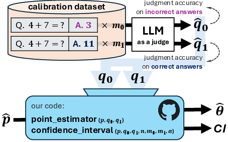
Calibrating the judge
To understand the judge’s mistakes, the authors use a small “calibration” dataset where humans have already decided what’s truly correct or incorrect. On that set, they measure:
- : the judge’s accuracy on truly correct answers
- : the judge’s accuracy on truly incorrect answers
These numbers tell us how the judge behaves in both situations.
Correcting the score
Suppose on your big test set, the judge says a fraction of answers are “correct.” If the judge were perfect, you could trust . But because the judge makes errors, the paper uses a classical correction to estimate the true accuracy :
- : what the judge said on the test set
- : what you measured on the calibration set
This “plug-in” formula removes the judge’s bias. If the judge is very reliable, the correction is small; if the judge is less reliable, the correction matters more.
Confidence intervals (the margin of error)
A good report needs a confidence interval (CI) to say how sure we are about . Here, uncertainty comes from two places:
- The test set (we only saw a sample of all possible questions).
- The calibration set (we estimated the judge’s accuracies).
The paper combines both sources to build a single CI around , using a well-established method for proportions that stays reliable even when sample sizes aren’t huge. In short: the CI is wider when either the test set is small or the calibration set is small, and it shrinks as you collect more data.
Choosing calibration sizes wisely (adaptive allocation)
Not all calibration examples help equally. The paper shows how to split your calibration budget between:
- examples that are truly incorrect (to estimate ), and
- examples that are truly correct (to estimate ),
so that the final CI is as short as possible. The idea:
- If the judge more often mislabels incorrect answers, spend more calibration on truly incorrect cases (improve ).
- If the test set has few correct answers, that also changes which side you should focus on.
They propose a simple “pilot” step: collect a small, balanced calibration sample, estimate and , and then allocate the rest of your calibration budget to the side that will shrink the CI most.
Main Results
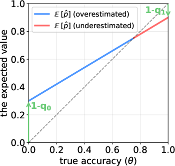
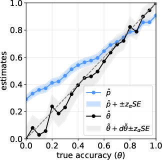
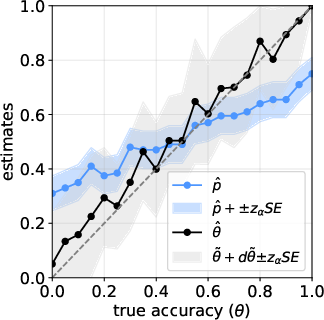
- The raw judge score (just “percent marked correct”) is biased when the judge isn’t perfect. It can overstate performance at low true accuracy and understate performance at high true accuracy.
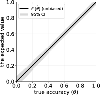
- The plug-in correction above removes most of that bias, giving a much more accurate estimate of the true accuracy against human judgement.
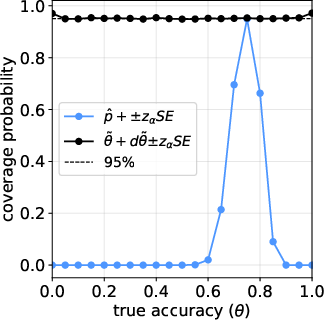
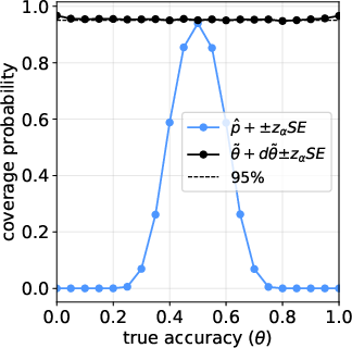
- The new confidence interval properly reflects uncertainty from both datasets (test and calibration) and achieves the intended coverage (for example, a 95% CI really covers the true accuracy about 95% of the time in simulations).
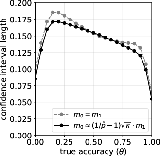
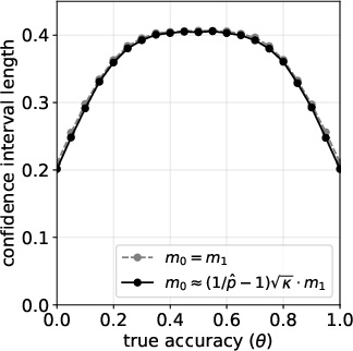
- The adaptive calibration strategy (how you split examples between truly correct and truly incorrect) consistently makes confidence intervals shorter compared to a simple 50/50 split.
- There’s a ready-to-use Python implementation so researchers can apply this easily.
Why It Matters
As more papers use LLMs to judge other models, reported improvements could be inflated or deflated by judge errors, not real progress. This paper gives a clear, practical fix:
- Correct the judge’s bias with a simple formula.
- Report a confidence interval that accounts for uncertainty from both the test and calibration data.
- Use an adaptive calibration plan to reduce the margin of error efficiently.
Following these steps makes model evaluations fairer, more trustworthy, and easier to compare across studies.
Knowledge Gaps
Knowledge gaps, limitations, and open questions
Below is a concise, actionable list of what the paper leaves missing, uncertain, or unexplored, to guide future research.
- Binary-only setting: Extend the framework beyond binary “correct/incorrect” judgments to multi-class labels, graded/continuous scores (e.g., scales, rubric sub-scores), and pairwise preferences (win rates), including corrected estimators and confidence intervals for each.
- Constancy of judge accuracy: Investigate models where judge sensitivity/specificity () vary with instance features, prompt templates, domains, or the system under evaluation; develop stratified or covariate-conditional calibration and corrections.
- Distribution shift: Quantify and correct for shifts between calibration and test distributions (including output-style shift across different SUTs), and provide sensitivity analyses or transportability guarantees when do not transfer.
- Dependence between datasets: Relax the assumption that test and calibration data are independent and identically distributed; derive variance/CI formulas that are robust to clustering, temporal dependence, or shared-source correlation.
- Judge drift over time: Develop procedures for monitoring and updating under model updates, API changes, prompt instruction revisions, or temperature changes, including sequential/online recalibration with guarantees.
- Imperfect “ground truth”: Model human label noise and annotator disagreement (e.g., latent class or Dawid–Skene-style models) and propagate this uncertainty through the bias correction and interval construction.
- Subgroup fairness: Estimate and report subgroup-specific (e.g., by topic, demographic attributes, input language), provide subgroup-aware corrections, and characterize fairness trade-offs in corrected accuracy.
- Comparative evaluation: Provide corrected estimators and CIs for differences between systems, rankings across many systems, and paired testing designs, accounting for correlation induced by using the same judge.
- Pairwise and ranking metrics: Generalize the approach to preference data (A/B tests, tournament win rates, rank aggregation), deriving misclassification-aware corrections and valid uncertainty quantification.
- Small-sample and boundary behavior: Analyze finite-sample coverage of the proposed Wald-type CI, especially when sample sizes are small, are extreme (near 0 or 1), or corrected estimates sit near the [0,1] boundaries; compare with exact, profile-likelihood, bootstrap, or Bayesian intervals.
- Truncation effects: Quantify the impact of truncating corrected estimates/CIs to [0,1] on bias and coverage; evaluate alternatives (e.g., logit-transformed intervals or constrained optimization).
- Overdispersion and correlated judge errors: Address overdispersion (e.g., beta-binomial/clustered errors) and topic/item-level dependencies that can make standard binomial variance understate uncertainty; propose cluster-robust or hierarchical variance estimators.
- Edge cases and stability: Provide diagnostics and safeguards when or close to 1 (ill-conditioned denominator), including regularization/shrinkage for estimates, conservative intervals, or decision rules for abandoning LLM-judge use.
- Optimal allocation beyond approximations: Analyze the adaptive allocation rule without the “ close to 1” assumption; provide non-asymptotic bounds and robustness to using biased and noisy pilot estimates in the allocation.
- Practical implementability of allocation: Address how to achieve target when the true label z is unknown before annotation; design sequential labeling workflows (e.g., screen-then-confirm) and quantify cost/benefit.
- Budgeted design: Develop closed-form/sample-size calculators for meeting target CI widths under joint constraints on test size n and calibration sizes m0, m1; incorporate monetary/time costs and propose optimal budget allocations.
- Prompting and protocol sensitivity: Study how judge prompt design, rubric specificity, chain-of-thought visibility, and multi-turn judging affect , and how to standardize or calibrate across protocols.
- Multiple judges and ensembling: Extend to settings with multiple LLM judges or human–LLM hybrids (e.g., majority vote, stacking), including joint estimation of judge-specific ’s and ensemble-level corrections/intervals.
- Multi-criteria evaluation: Generalize to vector-valued outcomes (e.g., helpfulness, harmlessness, factuality), including joint corrections, multiplicity control, and multivariate uncertainty reporting.
- Strategic behavior and adversarial robustness: Model systems that exploit judge weaknesses; design evaluation protocols and corrections minimizing worst-case bias under targeted attacks.
- Real-world validation: Apply the method to public LLM benchmarks with human ground truth to assess external validity, judge/version drift, subgroup effects, and the practical gains of adaptive allocation.
- Reuse and transfer of calibration: Determine when a calibration obtained on task A can be safely reused on task B or system B; formalize criteria and tests for calibration portability.
- Software robustness: Specify numerical stability safeguards (e.g., handling near-singular denominators, extreme proportions), default priors/shrinkage for estimation, and reproducibility standards in the provided implementation.
Practical Applications
Overview
The paper introduces a practical, statistically grounded framework for using LLMs as evaluators (“LLM-as-a-Judge”). It provides:
- A bias-corrected estimator for true accuracy using the judge’s sensitivity and specificity.
- A confidence interval that accounts for uncertainty from both test and calibration datasets.
- An adaptive calibration-sample allocation algorithm to minimize interval length under fixed budgets.
- A ready-to-use Python implementation: https://github.com/UW-Madison-Lee-Lab/LLM-judge-reporting.
Below are concrete applications across sectors and settings, organized by immediate and long-term horizons. Each item notes likely tools/workflows and key dependencies that impact feasibility.
Immediate Applications
These applications can be deployed now using the paper’s plug-in estimator, confidence intervals, and adaptive calibration design.
- Industry (Software): Calibrated LLM evaluator for code-generation quality gates
- Use case: Replace raw LLM-judge pass rates with bias-adjusted accuracy and 95% CI to gate model deployments (e.g., “merge if corrected accuracy ≥ target and CI width ≤ threshold”).
- Workflow:
- 1) Collect a small, human-labeled calibration set split into “correct” and “incorrect” code solutions.
- 2) Compute corrected accuracy and CI with the provided Python package.
- 3) Apply adaptive calibration to minimize CI length under budget.
- Dependencies/assumptions: Stable prompts/judge behavior; calibration labels reflect the target domain; binary correctness mapping; independence between test and calibration datasets.
- Industry (Trust & Safety): Confidence-aware LLM moderation filters
- Use case: Calibrate an LLM that flags harmful content; report corrected precision/recall proxies via ; set thresholds with CI-aware risk tolerance.
- Tools: The plug-in estimator + CI to set operational thresholds; dashboards to track judge drift and recalibration needs.
- Dependencies: Representative “harmful” vs “non-harmful” calibration labels; drift monitoring (judge reliability can change with new prompts/content); class imbalance handled via adaptive allocation.
- Industry (Product/UX Analytics): A/B testing of LLM features with bias-adjusted evaluation
- Use case: Compare model variants using corrected accuracy and overlapping CIs; avoid rollouts driven by judge bias.
- Workflow: Integrate the estimator into experimentation platforms (e.g., MLflow/W&B metrics), log corrected metrics and CI.
- Dependencies: Sufficient calibration size for desired CI length; consistent test distribution across variants.
- Academia (Benchmarking & Papers): Correct reporting of LLM-as-a-Judge results
- Use case: Replace naive “LLM says X% correct” with bias-adjusted estimates and CIs in publications and benchmarks.
- Tools: GitHub implementation; methods section specifying judge , calibration sampling plan, CI construction, and adaptive allocation.
- Dependencies: Availability of human-labeled calibration data; consistent judge prompts; clearly documented binary label mapping and truncation to [0,1].
- Benchmark Hosts/Leaderboards: Confidence-aware leaderboards for judged tasks
- Use case: Display corrected accuracy and uncertainty (CI width) for submissions judged by LLMs.
- Tools: “Confidence-aware leaderboard” module using the estimator and CI; flags for insufficient calibration (e.g., ).
- Dependencies: Governance for minimum calibration standards; periodic re-calibration; clear reporting of judge parameters and sample sizes.
- Education: Calibrated auto-grading for short answers/code exercises
- Use case: When an LLM acts as a grader, report corrected pass rates and CI; adapt calibration effort to reduce uncertainty for high-stakes assessments.
- Tools: Instructor dashboard integrating adaptive calibration allocation and CI reporting; policy for escalation to human grading when CI is too wide.
- Dependencies: Ground-truth rubric consistency; domain shift across assignments; student fairness considerations (documented judge reliability).
- Finance & Legal (Compliance Review): Evaluating LLM summaries/classifications with calibrated judges
- Use case: Use an LLM judge to assess whether generated reports meet compliance criteria; report corrected compliance rates with CI for auditability.
- Tools: Calibration on representative “compliant”/“non-compliant” documents; CI-aware thresholds for release decisions.
- Dependencies: High-quality, expert-labeled calibration data; tight domain focus; periodic reassessment under regulatory changes.
- Daily Life (LLM App Builders and Open-Source Maintainers): Trustworthy evaluation of app responses
- Use case: For productivity or Q&A apps that internally rely on an LLM judge, present corrected accuracy and uncertainty to users and contributors.
- Tools: Lightweight integration of the Python package; small pilot calibration to set initial judge parameters; adaptive allocation to improve confidence quickly.
- Dependencies: Willingness to collect a small number of human labels; maintaining stable judge prompts; clarity on what “correct/incorrect” means for the app.
Long-Term Applications
These require further research, standardization, scaling, or tooling maturation.
- Standards & Policy: Reporting requirements for LLM-as-a-Judge
- Use case: Publishers, funders, and standards bodies (e.g., ISO/IEC JTC 1/SC 42, NIST, ACM/ACL) adopt guidance mandating bias-adjusted estimates and CIs when LLMs are evaluators.
- Potential outcomes: Template sections in papers/model cards; minimum calibration budgets; judge drift monitoring policies.
- Dependencies: Community consensus; tooling support in benchmark platforms; reviewer training.
- Generalized Judging Beyond Binary: Graded rubrics, multi-class, and pairwise preferences
- Use case: Extend methods to ordinal scores (rubrics), multi-label tasks, and preference judgments (A vs B).
- Potential tools: Generalized estimators and CIs for non-binary judgments; preference calibration where “sensitivity/specificity” map to Bradley–Terry or Thurstone models.
- Dependencies: Statistical extensions; new calibration designs; robust assumptions for more complex judgment types.
- Judge Optimization & Selection: Choosing or training judges to maximize and minimize uncertainty
- Use case: Evaluate multiple LLM judges/prompts; select the one with best calibrated reliability or ensemble judges for improved specificity/sensitivity.
- Potential products: “Judge selection” toolkits; prompt governance and judge ensembling; meta-evaluation dashboards.
- Dependencies: Cost/latency constraints; reliable estimation of judge parameters across domains; fairness considerations.
- Continuous/Online Calibration with Drift Detection
- Use case: Maintain CI quality under changing distributions (topics, languages, adversarial inputs) by streaming calibration and automated alerts when shift.
- Potential workflows: Active learning to pick calibration samples likely to reduce CI; periodic recalibration cycles.
- Dependencies: Monitoring infrastructure; labeled feedback loops; budget for ongoing human labeling.
- Cross-Domain and Multilingual Fairness Audits
- Use case: Calibrate judges across demographics/languages/domains; report domain-specific corrected metrics and CIs to surface misalignment and bias.
- Potential tools: Stratified calibration and reporting; fairness dashboards overlaying corrected metrics.
- Dependencies: Representative calibration sampling; governance for subgroup reporting; ethical review.
- Platform Integrations: EvaluationOps in ML toolchains
- Use case: First-class support in ML platforms (MLflow, Weights & Biases, Hugging Face Evaluate) for bias-adjusted metrics and CI logging.
- Potential products: “Calibrated Judge SDK,” “Confidence-aware evaluation” plugins; CI width as a deployment KPI.
- Dependencies: API design; standardized metadata (judge prompt, calibration sizes, estimates); organizational buy-in.
- Procurement and Regulatory Compliance
- Use case: Government/enterprise procurement requires calibrated reporting for LLM-evaluated benchmarks; regulators accept CI-aware evidence for safety claims.
- Potential outcomes: Contractual clauses; compliance checklists; third-party audits leveraging corrected estimates.
- Dependencies: Legal frameworks; auditor expertise; sector-specific calibration requirements (e.g., healthcare safety thresholds).
- Cost-Aware Calibration Planning and Marketplaces
- Use case: Optimize calibration budgets across tasks/products; marketplaces for expert calibration labeling; automated allocation beyond the paper’s pilot-based heuristic.
- Potential tools: Budget planners that target CI length; integrated active sampling; shared calibration pools.
- Dependencies: Labeler availability; task variation; standard contracts and data governance.
Key Assumptions and Dependencies (Cross-Cutting)
- Calibration data quality: Requires human-verified labels that reflect the evaluation domain.
- Stability: Judge accuracy () depends on prompts, instructions, and context; changes require recalibration.
- Independence: Test and calibration datasets should be independent; leakage biases estimates.
- Binary mapping: The current estimator assumes binary correctness. Non-binary judgments need methodological extensions.
- Sample sizes: Desired CI width dictates calibration budget; adaptive allocation helps but cannot replace insufficient labeling.
- Distribution shift: If the test distribution differs materially from calibration, corrected estimates may misrepresent true accuracy; drift monitoring is important.
- Transparency: Report all judge settings, calibration sizes, and CI construction details to ensure reproducibility and trust.
By adopting the paper’s methods and tooling, organizations can improve the reliability, transparency, and comparability of LLM-based evaluations today, while laying the groundwork for standardized, fairness-aware judging practices in the future.
Glossary
- Adaptive allocation: A procedure that allocates calibration samples between label types to minimize confidence-interval length using pilot estimates. "we introduce an adaptive allocation procedure in Algorithm~\ref{alg:allocation}."
- Adjusted Wald interval: A corrected Wald confidence interval for proportions that adds pseudo-counts to improve coverage, often summarized as “add two successes and two failures.” "following the ``add two successes and two failures'' adjusted Wald interval approach"
- Asymptotic variance: The variance of an estimator in the large-sample limit, often derived via the delta method to construct approximate confidence intervals. "the asymptotic variance of is"
- Bias-adjusted estimator: An estimator that corrects bias due to judge misclassification by incorporating sensitivity and specificity (e.g., Rogan–Gladen style). "producing the bias-adjusted estimator ."
- Binomial distribution: The probability distribution modeling the number of successes in a fixed number of independent Bernoulli trials; used to derive variances of proportion estimates. "Because follows a binomial distribution"
- Calibration dataset: A labeled dataset with human ground-truth used to estimate the judge’s sensitivity and specificity parameters (, ). "they can be estimated from a calibration dataset with ground-truth labels"
- Confidence interval: An interval estimate that quantifies uncertainty about a parameter (here, true accuracy ), incorporating both test and calibration randomness. "and construct a confidence interval that accounts for uncertainty arising from both the test and calibration datasets"
- Coverage probability: The proportion of times a confidence interval contains the true parameter across repeated samples, used to assess interval reliability. "Fig.~\ref{fig:mc-simulation-cp} reports the empirical coverage probability of the confidence interval in~\eqref{eq:ci}."
- Delta method: A technique to approximate the variance of a function of estimators using a Taylor expansion, central to deriving the variance of . "By applying the delta method~\citep{dorfman1938note, ver2012invented}, the asymptotic variance of is"
- Error ratio: The ratio of error probabilities across label types, typically , used to guide optimal calibration allocation. "Compute the estimated error–ratio: ."
- Indicator function: A function that returns 1 if a condition holds and 0 otherwise, used to define empirical accuracies. "where denotes the indicator function."
- Law of total probability: A rule that decomposes probabilities across a partition, used here to relate observed judge predictions to true accuracy and judge accuracies. "By the law of total probability, we have"
- LLM-as-a-Judge: An evaluation paradigm where an LLM is used as the judge in place of humans to label correctness or quality. "LLM-as-a-Judge evaluation involves two sources of uncertainty:"
- Misclassification bias: Bias in an estimated accuracy arising from a judge’s false positives/negatives, which the adjustment aims to correct. "which exactly corrects for the LLMâs misclassification bias."
- Monte Carlo simulation: A computational experiment using repeated random sampling to assess estimator bias, coverage, and interval length. "Monte Carlo simulation for estimating under an imperfect LLM judge with ."
- Pilot calibration sample: A small initial calibration set used to estimate judge accuracies and inform adaptive allocation of the full calibration budget. "The algorithm begins by collecting a small pilot calibration sample (e.g., $m_{\mathrm{pilot} = 10$ for each label type)"
- Plug-in estimator: An estimator obtained by substituting estimated nuisance parameters (e.g., , ) into a correction formula. "derive a simple plug-in estimator that corrects the resulting bias"
- Prevalence estimation: Estimating the true proportion of positives corrected for imperfect tests, providing the classical basis for the bias adjustment. "a classical result from prevalence estimation \citep{rogan1978estimating} provides an exact adjustment."
- Quantile (standard normal): The value cutting off a specified upper tail probability of the standard normal distribution, used to set confidence-level multipliers. " denotes the quantile of the standard normal distribution"
- Sensitivity: The judge’s true positive rate, , i.e., probability of marking a truly correct item as correct. "where and are LLMâs sensitivity and specificity."
- Specificity: The judge’s true negative rate, , i.e., probability of marking a truly incorrect item as incorrect. "where and are LLMâs sensitivity and specificity."
- Wald-type confidence interval: A confidence interval based on a normal approximation using the estimator’s variance, here applied after adjustments to improve coverage. "yields the Wald-type confidence interval shown in \eqref{eq:ci}"
Collections
Sign up for free to add this paper to one or more collections.