Generative Modeling via Drifting
Abstract: Generative modeling can be formulated as learning a mapping f such that its pushforward distribution matches the data distribution. The pushforward behavior can be carried out iteratively at inference time, for example in diffusion and flow-based models. In this paper, we propose a new paradigm called Drifting Models, which evolve the pushforward distribution during training and naturally admit one-step inference. We introduce a drifting field that governs the sample movement and achieves equilibrium when the distributions match. This leads to a training objective that allows the neural network optimizer to evolve the distribution. In experiments, our one-step generator achieves state-of-the-art results on ImageNet at 256 x 256 resolution, with an FID of 1.54 in latent space and 1.61 in pixel space. We hope that our work opens up new opportunities for high-quality one-step generation.

Paper Prompts
Sign up for free to create and run prompts on this paper using GPT-5.
Top Community Prompts
Explain it Like I'm 14
Overview
This paper introduces a new way to train image generators called Drifting Models. The big idea is simple: while training, gently “push” fake samples toward real ones in a smart way, so that when training is done, the model can create a whole image in a single step. Unlike diffusion models, which clean up noise over tens or hundreds of steps, Drifting Models generate in one go.
What is the paper trying to do?
The authors set out to answer a few easy-to-understand questions:
- Can we train a generator that makes high‑quality images in one step, instead of many?
- Can we guide the model during training using a clear, non-adversarial rule that says how fake samples should move to look more like real data?
- Can this approach match or beat the best one-step methods, and compete with multi-step methods?
How does it work? (Everyday explanation)
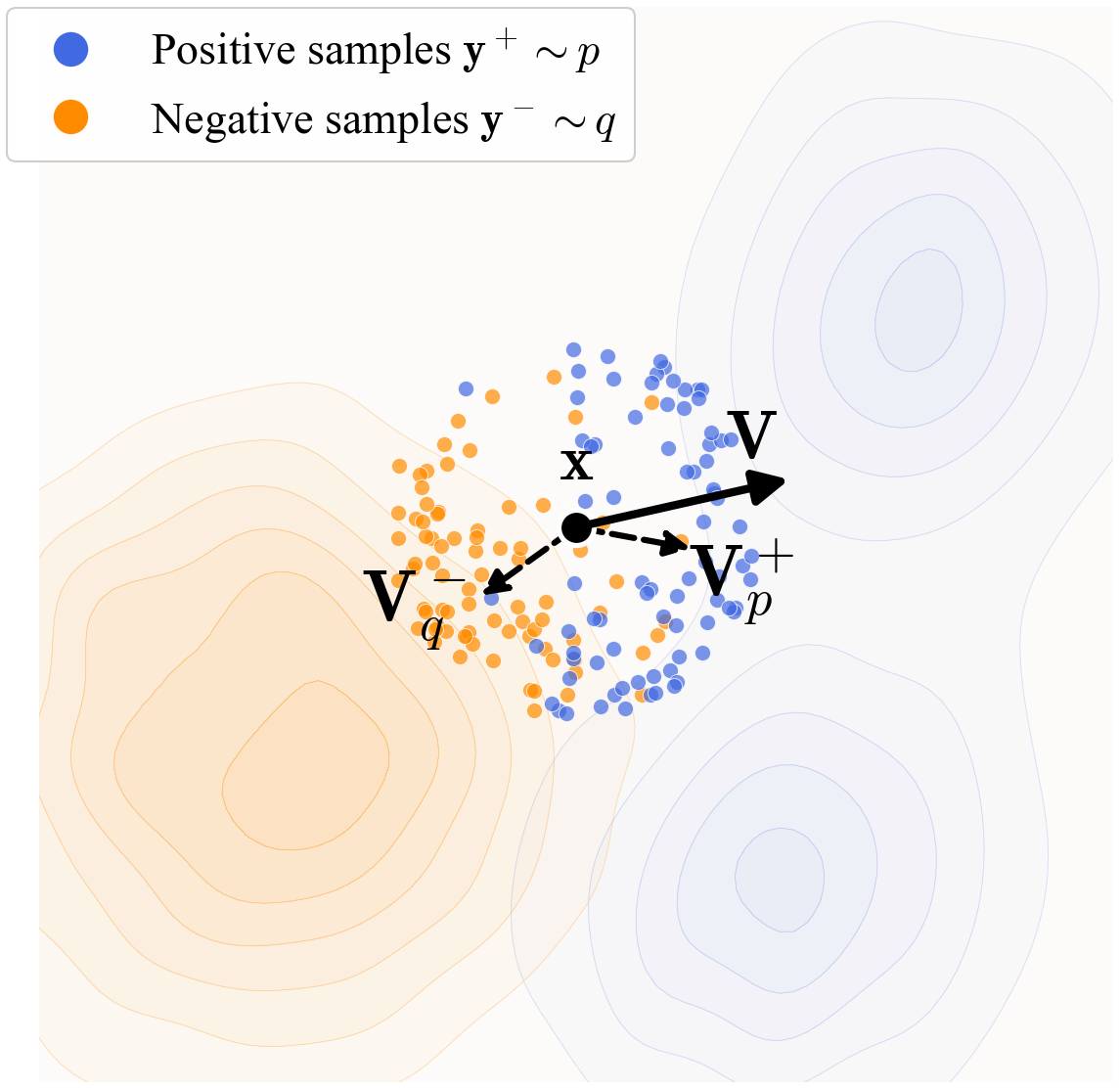
Think of all real images as blue dots sprinkled in space, and the model’s current fake images as orange dots. The goal is to move the orange dots so they line up with the blue ones.
Here are the key parts:
- Distributions as “shapes”: A distribution is just the shape of where samples tend to be. The real images form the real-data shape. The model turns random noise into fake images, forming the model’s shape.
- Drifting field (the “how to move” rule): For each fake sample, the model computes a little arrow showing which way to move it. This arrow is called the drift. It is built from two forces:
- Attraction to real images: pull the fake sample toward nearby real samples.
- Repulsion from fake images: push it away from nearby fake samples to avoid crowding or mode collapse.
When the fake and real distributions match perfectly, the attraction and repulsion cancel out for every point—so the drift is zero. That’s “equilibrium.”
- How do we measure “nearby”? The model uses a similarity function (a “kernel”) that gives higher weight to real or fake samples that look similar. To make “similarity” meaningful, they don’t compare raw pixels. Instead, they pass images through a feature encoder (a network trained to understand image content) so images with similar content are close in that feature space.
- Training step (the “move toward where the arrow points” trick): At each training iteration, the model:
- Generates a batch of fake images.
- Looks at a batch of real images.
- Computes the drift arrows in feature space: attract to reals, repel from fakes.
- Treats the “drifted” positions as a temporary target and updates the generator so its outputs move in that direction.
The loss the model minimizes is basically “how long the arrows are.” Shorter arrows mean the fake and real distributions are closer. When arrows shrink to zero, you’ve matched the real data.
Why does one-step generation work? All the “stepping” (the small movements guided by the arrows) happens during training. By the end, the generator has learned to map noise directly to realistic images in one pass. At inference time, there’s no need to iterate.
Class-conditional guidance (CFG) made simple: For class-labeled images (like “dog,” “car,” etc.), they adapt their drifting to be stronger for the desired class by mixing in “negatives” from other classes while training. This plays a similar role to classifier-free guidance in diffusion models, but it stays one-step at test time.
What did they find?
Strong one-step image generation:
- On ImageNet at 256×256 resolution:
- Latent-space generation: FID 1.54 (lower is better), which is state-of-the-art among one-step methods and competitive with multi-step methods.
- Pixel-space generation (no latent tokenizer): FID 1.61, again very strong and better than many multi-step methods.
- One-step means NFE=1 (number of function evaluations/steps is one).
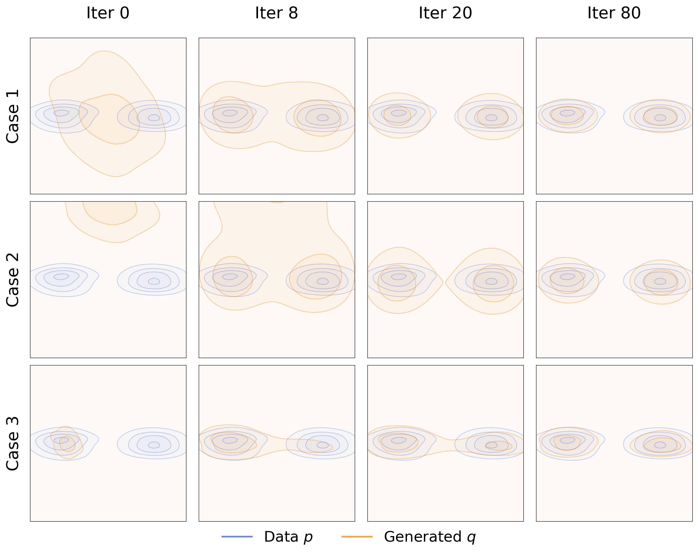
- No mode collapse in toy examples: In simple 2D tests (think dots on a plane), the method spreads out properly and covers all “modes” of the data, even if it starts collapsed on one mode. The attraction–repulsion design helps avoid collapse.
- The anti-symmetry property matters: If you break the balance between attraction and repulsion, performance falls apart. This balance is key to reaching equilibrium.
- More (and better) examples improve learning: Using more positive (real) and negative (fake) samples per batch gives a better estimate of the drift and improves quality.
- Feature space quality is crucial: Better feature encoders (like a specially trained latent-space MAE) help a lot because they make the similarity measure more meaningful, which makes the drift smarter.
- Beyond images: In robotics control benchmarks, replacing a 100‑step diffusion policy with a one-step drifting policy matched or beat performance on several tasks. This shows the idea is not limited to images.
What are FID and IS? FID is a common score for image quality and diversity: lower is better. IS (Inception Score) is another measure where higher is better.
Why is this important?
- Speed: One-step generation is fast and efficient, which is great for real-time apps, mobile devices, or any setting where speed and cost matter.
- Simplicity: It avoids complex multi-step solvers at inference time and does not rely on adversarial training like GANs.
- Generality: The drifting idea applies to different data types (images, control actions) and could be extended further.
Final thoughts and impact
Drifting Models offer a fresh way to think about generative learning: use training time to evolve the model’s output distribution until attraction and repulsion balance out. The result is a generator that creates high-quality outputs in a single step. While there are open theory questions—like exactly when “zero drift” guarantees a perfect match—the strong results on ImageNet and robotics suggest this paradigm is both practical and promising. It could inspire faster, simpler generative systems across many domains, from creative tools to robotics and beyond.
Knowledge Gaps
Knowledge gaps, limitations, and open questions
Below is a concise list of what remains missing, uncertain, or unexplored in the paper, written to be concrete and actionable for future research:
- Formal convergence guarantees: characterize conditions (on the kernel k, feature encoder φ, prior distribution, and optimizer) under which minimizing the drift loss leads to q→p; provide proofs that V≈0 implies q≈p in high-dimensional settings and derive convergence rates.
- Spurious equilibria and identifiability: systematically identify scenarios where V≈0 but q≠p (e.g., flat kernels, degenerate supports, feature collapse) and develop diagnostics or regularizers to avoid trivial equilibria.
- Dynamics and stability analysis: analyze the training-time drift dynamics x_{i+1}=x_i+V(x_i) with stop-gradient targets, including stability, step-size sensitivity, overshoot conditions, and guarantees against collapse; determine how optimizer hyperparameters influence equilibrium.
- Kernel design and normalization: evaluate alternative kernels (e.g., Gaussian RBF, cosine similarity, learned metrics), anisotropic or data-adaptive kernels, and different normalization schemes (softmax over y, over x, or none); provide principled criteria for choosing τ and scheduling it during training.
- Anti-symmetry sufficiency: explore whether anti-symmetry alone is sufficient for good behavior or if stronger structural conditions on V (e.g., monotonicity, conservative fields) are needed; prove whether the extra softmax normalization over x preserves anti-symmetry in all cases.
- Feature-space dependence: explain why the method fails on ImageNet without a feature encoder; determine when matching φ#q to φ#p is sufficient to match q to p in pixel space, and when it is not; study bias and domain shift induced by pre-trained φ and the effects of fine-tuning φ jointly with the generator.
- Learning φ end-to-end: investigate joint training or adaptation of the feature extractor (instead of relying solely on frozen SSL encoders) and quantify trade-offs between representation quality, drift signal richness, stability, and overfitting risks.
- Positive/negative sampling strategy: establish scaling laws and optimal allocation of N_pos and N_neg under fixed compute; explore cross-batch memory banks, momentum queues, hard-negative mining, class-balanced sampling, and curriculum strategies; quantify impacts on diversity and precision.
- Computational complexity and scalability: measure and reduce the O(B·N_pos·N_neg) kernel interaction cost; investigate approximate nearest neighbor search, locality-sensitive hashing, attention pruning, or sparse kernels; assess scaling to higher resolutions (e.g., 512×512, 1024×1024).
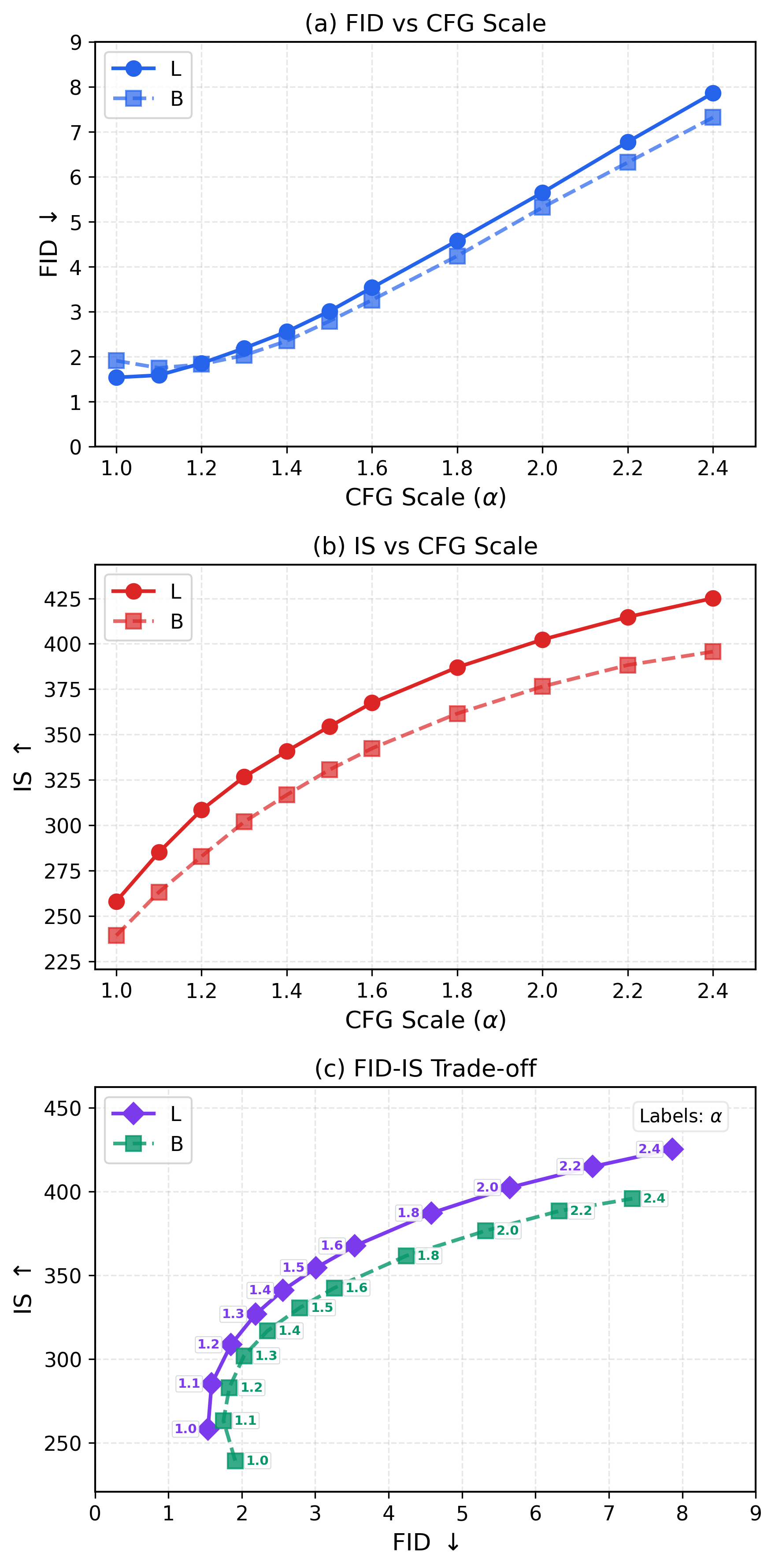
- CFG as training-time guidance: provide a theoretical justification for the mixture in Eq. (cfg1–cfg2); analyze how γ/α choices bias the learned conditional and unconditional generators; quantify label leakage, class mixing artifacts, and the FID/IS trade-off versus inference-time CFG.
- Relation to MMD/contrastive objectives: formally connect the drift loss E[||V||2] to MMD or other IPM metrics under specific kernels; derive bounds, equivalences, or separations; compare empirically to MMD training with characteristic kernels.
- Generator architecture generality: test beyond DiT-like backbones (e.g., CNNs/UNets, autoregressive, invertible flows) and different patch sizes; evaluate effects of input/output dimensionality mismatches (C≠D) and priors other than Gaussian.
- Tokenizer/decoder dependence: quantify how fixed SD-VAE (or VA-VAE/RAE) tokenizers impact performance; compare pixel-space vs. various latent-space tokenizers; assess whether joint training of tokenizer/decoder improves drift signal or stability.
- Metrics beyond FID/IS: evaluate precision/recall, diversity/memorization, CLIP score, per-class breakdowns, long-tail coverage, and OOD generalization; provide human evaluations and robustness analyses to confirm absence of mode collapse at ImageNet scale.
- Robustness and safety: study sensitivity to feature encoder biases, adversarial perturbations, corruptions, and fairness concerns; assess calibration and reliability under distribution shift.
- Domain generalization: extend drifting models to text, audio, molecules, and discrete/token spaces; design appropriate kernels for discrete or structured data; evaluate conditional generation beyond class labels (e.g., text prompts).
- Sample complexity and generalization: derive how many positives/negatives are needed for reliable estimation of V; provide generalization bounds for the empirical drift estimates under mini-batch training.
- Training efficiency and wall-clock: report training time, throughput, and energy vs. diffusion/flow baselines; analyze diminishing returns with very long training (up to 1280 epochs) and propose schedules or curricula that improve efficiency.
- Step-size control of drift: investigate explicit scaling of V (learned or scheduled) to control drift magnitude, reduce instability, and accelerate convergence; compare to implicit control via the MSE loss.
- Backprop through V: explore alternatives to stop-gradient (e.g., implicit differentiation, bilevel/implicit objectives, score-function estimators) and quantify benefits/risks in variance, bias, and stability.
- Why robotics worked without φ: explain why raw representations suffice for control tasks but not for high-dimensional images; determine conditions under which feature-free drifting is viable and whether task-specific encoders help.
- Conditioning beyond classes: extend drifting guidance to continuous or multi-modal conditions (text, style, attributes); design mixtures of negatives/positives tailored to complex conditioning.
- Identifiability in high dimensions: formalize “mild non-degeneracy” assumptions under which bilinear constraints enforce q≈p; evaluate characteristic kernels in feature space and address the curse of dimensionality.
- Controlling inference diversity: study mechanisms to control sample diversity beyond the noise draw (e.g., temperature, truncation, guidance scaling) in one-step generation; quantify diversity-quality trade-offs.
- Reproducibility of compute_V: provide full derivations and proofs for implementation choices (e.g., batch-wise normalizations, masking, multi-scale features) and their theoretical properties (anti-symmetry, unbiasedness).
Practical Applications
Overview
This paper introduces Drifting Models, a one-step generative modeling paradigm that evolves the pushforward distribution during training via an anti-symmetric “drifting field.” It achieves state-of-the-art one-step image generation on ImageNet 256×256 (FID 1.54 in latent space; 1.61 in pixel space) and shows promising results when replacing Diffusion Policy in robotics with a one-step “Drifting Policy.” The method is practical for production due to reduced inference cost and latency, and its training-time dynamics open new tools for monitoring and designing generative systems.
Below are practical applications organized by timeline and use context, with sector tags, suggested tools/workflows, and key assumptions/dependencies.
Immediate Applications
These applications can be deployed now with modest adaptation of existing pipelines.
- One-step image generation for production pipelines
- Sector: software, media, advertising, e-commerce
- Use case: Replace multi-step diffusion/flow generators with Drifting Models to reduce inference latency and cost for product imagery, ads, catalog generation, and creative assets.
- Tools/workflows:
- Train a DiT-like one-step generator with SD-VAE tokenizer (latent space) or pixel-space variant (DiT/16).
- Use a high-quality self-supervised feature encoder (e.g., MoCo, SimCLR, or the paper’s latent-MAE) for training-time drifting loss.
- Implement the provided compute_V kernelized drift, with anti-symmetric V, multi-scale feature losses, and CFG-conditioning (training-time only).
- Monitor drift-norm (||V||²) and FID/IS during training; tune N_pos/N_neg, τ (temperature), and batch sizes to stabilize training.
- Assumptions/dependencies: Requires access to labeled/conditional data for CFG, strong feature encoders for high-dimensional content, and sufficient training compute; inference is one-step and lightweight.
- Mobile and edge deployment of generative features
- Sector: consumer tech, AR/VR, camera apps
- Use case: Real-time photo stylization, avatars, and filters on device with one-step inference, lowering energy and latency compared to multi-step diffusion.
- Tools/workflows: Pixel-space Drifting Model (DiT/16), post-training quantization or distillation to fit device constraints; optional latent-space generation if a tokenizer fits device memory.
- Assumptions/dependencies: Feature encoder is only used at training; inference must meet memory/compute budgets; potential need for model compression.
- Robotics control with one-step “Drifting Policy”
- Sector: robotics, automation, industrial manipulation
- Use case: Replace multi-step Diffusion Policy with Drifting Models to achieve similar or better success rates with 1-NFE in single- and multi-stage tasks (e.g., Lift, Can, ToolHang, PushT, BlockPush, Kitchen).
- Tools/workflows: Train the generator on demonstration datasets; compute drift directly on raw state/action representations (no feature encoder required for these tasks); integrate into control loop.
- Assumptions/dependencies: Requires sufficient demonstration data and careful tuning of V; tested scope covers common benchmarks—additional validation needed for safety-critical deployments.
- High-throughput synthetic data generation and augmentation
- Sector: healthcare, finance, autonomous driving, retail
- Use case: Create realistic synthetic images or state-action sequences to augment datasets, accelerate model training, and reduce privacy exposure.
- Tools/workflows: Train one-step generators per domain; rapidly generate large volumes of samples; track ||V||² and statistical metrics (FID/IS or domain-specific measures).
- Assumptions/dependencies: Validate synthetic data utility and privacy claims; ensure domain-appropriate quality metrics and bias checks.
- Fast creative iteration and A/B testing
- Sector: marketing, design
- Use case: Quick variants for creatives and campaigns; integrate a CFG scale slider to trade-off FID and IS on the fly without retraining.
- Tools/workflows: Class-conditional training with CFG-conditioning; productized inference API exposing class label and CFG scale; latency-critical serving.
- Assumptions/dependencies: Requires class labels or other conditioning signals; ensure content safety guidelines.
- Training-time diagnostics and stability monitoring
- Sector: academia, ML engineering
- Use case: Use the drift norm (||V||²) as an interpretable proxy for distribution mismatch; detect mode collapse (via low movement) and adjust kernel temperature, N_pos/N_neg, or feature encoder quality.
- Tools/workflows: Monitoring dashboards; ablations over kernel functions and normalizations; anti-symmetry checks; multi-scale feature losses.
- Assumptions/dependencies: Drift-norm correlates with quality but is not a formal guarantee; feature-space choice is critical.
- Drop-in module for diffusion/flow pipelines
- Sector: AI platform/infrastructure
- Use case: Replace multi-step generator blocks with one-step Drifting Models while retaining existing tokenizers, decoders, and conditional controls.
- Tools/workflows: Keep SD-VAE or pixel decoders; refactor pipeline to compute training-time drift in feature space; maintain CFG at training, 1-NFE inference at serving.
- Assumptions/dependencies: Requires re-training; pipelines must accommodate new training losses; compatibility testing with existing post-processing steps.
- Energy and cost reduction for generative services
- Sector: cloud, sustainability
- Use case: Achieve substantial inference FLOP reductions (e.g., 87G vs 1574G in comparisons) by eliminating 50–100+ NFE loops; reduce serving costs and carbon footprint.
- Tools/workflows: Track cost/energy metrics; capacity planning for one-step inference; cost modeling and ROI analysis.
- Assumptions/dependencies: Comparable output quality for target use cases; training cost and migration effort considered in total cost of ownership.
- Rapid research prototyping of kernelized drift and feature spaces
- Sector: academia, R&D labs
- Use case: Explore kernel choices, InfoNCE-like softmax normalizations, multi-scale drifting, and anti-symmetric fields as alternatives to ODE/SDE trajectories.
- Tools/workflows: Reference implementation of compute_V; plug-and-play feature encoders; toy experiments; robust logging of drift-norm vs FID/IS.
- Assumptions/dependencies: Hyperparameter sensitivity and compute demands; reproducibility under different datasets.
- Real-time interactive content in games and XR
- Sector: gaming, metaverse, XR
- Use case: One-step generation of textures, avatars, and scene assets for in-game customization and live events.
- Tools/workflows: Engine integration (Unity/Unreal); pixel- or latent-space models; low-latency inference endpoints.
- Assumptions/dependencies: IP/licensing for training data; meeting platform performance budgets; safety filters.
Long-Term Applications
These opportunities require further research, scaling, or development.
- Cross-modal one-step generation (audio, video, text)
- Sector: media, assistive tech, communications
- Use case: Extend drifting to audio synthesis, video generation, and possibly discrete tokens (text) by adopting domain-specific feature encoders (wav2vec, video SSL, language representations).
- Tools/workflows: Redesign generators for temporal/sequential data; adapt kernels and normalization; evaluate with domain metrics (PESQ, FVD, BLEU).
- Assumptions/dependencies: Availability of strong SSL encoders; theoretical and empirical validation for discrete/temporal modalities.
- Theoretical guarantees and safety frameworks
- Sector: academia, policy, safety
- Use case: Establish conditions where V→0 implies q→p; develop fairness and robustness criteria for drift fields; certify safety for regulated domains.
- Tools/workflows: Identifiability analysis of kernelized fields; fairness audits; adversarial drift stress tests; safety benchmarks.
- Assumptions/dependencies: Mathematical progress on distribution matching via drift; community consensus on evaluation protocols.
- Domain-specific one-step generation for medical and scientific imaging
- Sector: healthcare, pharma, remote sensing
- Use case: Rapid synthetic MRIs/CTs, microscopy, or satellite imagery for training and simulation; real-time augmentation during model development.
- Tools/workflows: Use SSL medical encoders (e.g., MoCo for radiology); calibrate kernels; domain-specific validation (clinical utility, radiologist studies).
- Assumptions/dependencies: Regulatory compliance (HIPAA/GDPR); rigorous bias and hallucination evaluation; expert sign-off.
- Edge robotics and IoT policies
- Sector: industrial automation, logistics
- Use case: One-step policies for on-device control enable faster cycle times and reduce dependency on cloud inference; potential for task chaining using multi-stage drifting.
- Tools/workflows: Composable training strategies across task phases; runtime resource caps; hybrid controllers with safety fallbacks.
- Assumptions/dependencies: Reliability under distribution shift; certification for industrial environments.
- Generative compression and tokenization
- Sector: telecom, streaming, storage
- Use case: One-step generative decoders/tokenizers to reduce bandwidth and decode latency; integrate with VAEs or RAEs.
- Tools/workflows: Design rate–distortion optimized drifting decoders; evaluate streaming QoE; server–client model alignment.
- Assumptions/dependencies: Competitive bitrate/quality trade-offs; efficient on-device decoding; ecosystem support.
- Green AI procurement and standards
- Sector: policy, enterprise IT
- Use case: Encourage adoption of low-NFE generative models through energy-aware benchmarks and procurement guidelines; standardize reporting on drift-norm and energy per sample.
- Tools/workflows: Carbon accounting frameworks; energy labels for AI services; internal governance aligning model selection with sustainability goals.
- Assumptions/dependencies: Robust cross-domain quality metrics; stakeholder buy-in; harmonization with existing regulations.
- Feature encoder marketplaces and ecosystem
- Sector: AI tooling
- Use case: Curate, license, and maintain domain-tuned SSL encoders optimized for drifting; offer evaluation dashboards and plug-ins.
- Tools/workflows: Packaging of encoders with kernel presets; benchmarking suites; SDK integration layers.
- Assumptions/dependencies: IP/licensing clarity; consistent performance across datasets; security and update practices.
- AutoML for drift-field design
- Sector: ML platforms, MLOps
- Use case: Automated search over kernel functions, τ, normalization strategies, and multi-scale loss weights to maximize quality under compute budgets.
- Tools/workflows: HPO pipelines; meta-learning; ablation harness integrated with drift-norm and target metrics.
- Assumptions/dependencies: Cost-effective search; generalizability across domains; reproducibility.
- Security and adversarial robustness via drift-aware training
- Sector: cybersecurity
- Use case: Use anti-symmetric repulsion to push away known adversarial or spam distributions during training; create generative defenses complementary to discriminative filters.
- Tools/workflows: Negative sampling from attack distributions; kernel/temperature tuning for robustness; joint training with classifiers.
- Assumptions/dependencies: Empirical efficacy; formal guarantees pending; careful evaluation to avoid unintended bias.
- EdTech and offline learning tools
- Sector: education
- Use case: Lightweight, offline generative assistants producing diagrams, exercises, and visualizations on student devices; use drift-norm as a teaching aid for understanding distribution matching.
- Tools/workflows: Classroom kits; Jupyter notebooks with toy drifting demos; curated datasets for safe content generation.
- Assumptions/dependencies: Device capabilities; content safety; teacher training and curriculum alignment.
Cross-cutting assumptions and dependencies
- Strong feature encoders are critical for high-dimensional domains; performance may degrade without them.
- Anti-symmetric drift must be preserved; destructive variants lead to failure.
- Larger positive/negative sample sets (N_pos, N_neg) improve drift estimation but raise training cost; inference remains one-step.
- Equilibrium condition (V≈0) empirically correlates with quality, but theoretical converse (V→0 ⇒ q→p) is not guaranteed in general.
- CFG is applied at training time; inference remains 1-NFE but depends on having appropriate class-conditional data for training.
- Tokenizers (e.g., SD-VAE) improve latent-space generation; pixel-space is feasible but may need different architectures and feature encoders.
- Ethical, legal, and safety reviews are necessary for sensitive sectors (healthcare, finance), especially when using synthetic data.
Glossary
- AdaLN-zero: A conditioning technique that initializes adaptive LayerNorm to zero so conditioning is learned stably. "Our model uses adaLN-zero for processing class-conditioning or other extra conditioning."
- Anti-symmetry: A property where swapping two arguments flips the sign; here, ensuring the drift field satisfies V_{p,q} = −V_{q,p}. "Consider an anti-symmetric drifting field:"
- Bilinear constraints: Constraints that are linear in each variable set separately; here, relations on distributions p and q implied by zero drift. "the zero-drift condition imposes a large set of bilinear constraints on (p,q)"
- Classifier-free guidance (CFG): A technique that improves conditional generation by combining conditional and unconditional predictions. "Classifier-free guidance (CFG) improves generation quality by extrapolating between class-conditional and unconditional distributions."
- Contrastive learning: A paradigm that learns representations by bringing positives closer and pushing negatives apart. "This is conceptually related to the positive and negative samples in contrastive representation learning"
- Diffusion models: Generative models that transform noise to data via stochastic/deterministic differential equations over multiple steps. "Diffusion models (e.g, \citealt{sohl2015deep,ho2020denoising,song2020score}) and their flow-based counterparts ... formulate noise-to-data mappings through differential equations (SDEs or ODEs)."
- DiT: Diffusion Transformer, a transformer-based architecture for image generation. "Our generator () has a DiT-like ... architecture."
- ELBO (Evidence Lower Bound): A variational objective decomposed into reconstruction and KL terms, optimized by VAEs. "VAEs optimize the evidence lower bound (ELBO), which consists of a reconstruction loss and a KL divergence term."
- Equilibrium: The state where the generated and data distributions match and the drift vanishes. "We introduce a drifting field that governs the sample movement and achieves equilibrium when the distributions match."
- Euler solver: A numerical integrator for ODEs used to step iterative update rules during sampling. "such as with an Euler solver."
- Feature space: A representation space produced by an encoder in which similarities and losses are computed. "Our formulation can be extended to any feature space."
- FID (Fréchet Inception Distance): A metric measuring similarity between generated and real image distributions using pretrained features. "we obtain a 1-NFE FID of 1.54 under the standard latent-space generation protocol"
- Fixed-point iteration: An iterative procedure seeking x = F(x); here used to align outputs with their drifted targets. "This equation motivates a fixed-point iteration during training."
- Flow Matching: A training framework that learns vector fields to transport distributions, related to continuous normalizing flows. "Flow Matching"
- Identifiability: The property that a model’s parameters/distributions are uniquely determined by observed criteria. "we provide an identifiability heuristic"
- InfoNCE: A contrastive loss based on normalized exponentiated similarities. "This softmax operation is similar to that of InfoNCE in contrastive learning."
- IS (Inception Score): A metric assessing image quality and diversity using a classifier’s outputs. "a tradeoff between FID and IS"
- Jacobian: The matrix of partial derivatives; its log-determinant is needed for likelihoods in normalizing flows. "These methods require invertible architectures and computable Jacobians."
- Kernel (similarity function): A function measuring similarity between samples, used to weight interactions in the drift. "The kernel k(·, ·) can be a function that measures the similarity."
- KL divergence: A measure of discrepancy between two probability distributions. "a KL divergence term."
- Latent space: A compressed representation space (e.g., VAE latents) where generation can be performed efficiently. "By default, we perform generation in latent space"
- MAE (Masked Autoencoder): A self-supervised pretraining method that reconstructs masked inputs, used here as a feature encoder. "We also study an MAE pre-trained in latent space"
- Maximum Mean Discrepancy (MMD): A kernel-based distance between distributions used for moment matching. "Moment-matching methods seek to minimize the Maximum Mean Discrepancy (MMD) between the generated and data distributions."
- Mean-shift: A mode-seeking procedure using kernel-weighted means; here it inspires attraction/repulsion drift vectors. "We define the following fields inspired by the mean-shift method"
- NFE (Number of Function Evaluations): The count of network evaluations needed at inference; 1-NFE denotes single-step generation. "Drifting Models naturally perform single-step (“1-NFE”) generation"
- Normalizing Flows (NFs): Likelihood-based generative models that use invertible mappings with tractable Jacobians. "NFs learn mappings from data to noise and optimize the log-likelihood of samples."
- ODE (Ordinary Differential Equation): A deterministic differential equation; used to describe sampling trajectories in some generative models. "differential equations (SDEs or ODEs)"
- Perceptual loss: A loss computed in feature space comparing representations rather than pixels. "Our feature-space loss is related to perceptual loss"
- Pushforward (f_#): The transformation of a distribution through a function; f_# p denotes the distribution of f(x) when x ~ p. "Here, ``" denotes the pushforward induced by ."
- Pushforward distribution: The distribution obtained by applying a mapping to samples from another distribution. "q is referred to as the pushforward distribution of p_ under f"
- SDE (Stochastic Differential Equation): A differential equation with stochastic terms; used to model diffusion processes. "differential equations (SDEs or ODEs)"
- Softmax: A normalization function turning logits into a probability distribution, used to implement normalized kernels. "we implement using a softmax operation"
- Stop-gradient: An operation that prevents backpropagation through a tensor, treating it as a constant target. "the stop-gradient operation provides a frozen state from the last iteration"
- Tokenizer: A learned encoder/decoder (e.g., VAE) that maps images to a compact latent code for generation. "We adopt the standard SD-VAE tokenizer"
- VAE (Variational Autoencoder): A generative model trained by maximizing the ELBO with an encoder–decoder architecture. "VAEs optimize the evidence lower bound (ELBO)"
Collections
Sign up for free to add this paper to one or more collections.