Flow Sampling: Learning to Sample from Unnormalized Densities via Denoising Conditional Processes

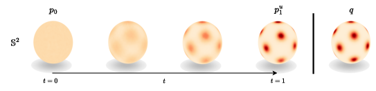
Abstract: Sampling from unnormalized densities is analogous to the generative modeling problem, but the target distribution is defined by a known energy function instead of data samples. Because evaluating the energy function is often costly, a primary challenge is to learn an efficient sampler. We introduce Flow Sampling, a framework built on diffusion models and flow matching for the data-free setting. Our training objective is conditioned on a noise sample and regresses onto a denoising diffusion drift constructed from the energy function. In contrast, diffusion models' objective is conditioned on a data sample and regresses onto a noising diffusion drift. We utilize the interpolant process to minimize the number of energy function evaluations during training, resulting in an efficient and scalable method for sampling unnormalized densities. Furthermore, our formulation naturally extends to Riemannian manifolds, enabling diffusion-based sampling in geometries beyond Euclidean space. We derive a closed-form formula for the conditional drift on constant curvature manifolds, including hyperspheres and hyperbolic spaces. We evaluate Flow Sampling on synthetic energy benchmarks, small peptides, large-scale amortized molecular conformer generation, and distributions supported on the sphere, demonstrating strong empirical performance.

• The paper introduces Flow Sampling, a diffusion-based method that leverages closed-form conditional denoising drifts to sample from unnormalized densities, reducing simulation cost by up to 8x.
• It integrates flow matching with Riemannian geometry extensions, enabling efficient sampling on manifolds and high-dimensional, multimodal landscapes.
• Empirical evaluations demonstrate state-of-the-art performance in molecular conformer generation and synthetic energy benchmarks compared to traditional MCMC approaches.

Sampling Unnormalized Densities with Flow Sampling: A Conditional Denoising Diffusion Framework

Introduction and Motivation

Sampling from unnormalized densities is a fundamental challenge in computational physics, chemistry, and Bayesian inference, where target distributions are specified only up to a normalization constant, and obtaining samples directly is infeasible due to the high cost of evaluating the energy or reward function. Classical algorithms such as MCMC and Langevin dynamics, while asymptotically exact, often suffer from slow mixing and limited scalability in high-dimensional or multimodal settings. Recent developments have used diffusion models and flow matching for amortized and accelerated sampling, but most approaches require either auxiliary MCMC steps, repeated score evaluations, or stochastic corrections, all of which significantly increase computational costs. The presented work introduces Flow Sampling, an efficient, data-free, diffusion-based sampling method that directly leverages the energy function, achieves high performance even for complex geometries, and provides an explicit extension to Riemannian manifolds (2605.03984).

Methodology

Flow Sampling Framework

Flow Sampling is motivated by the success of flow matching (FM) in generative modeling, where a velocity field is learned such that a time-evolving process interpolates between a tractable source distribution and a target. In the standard FM setting, the regression target is constructed using samples from the target; however, in the data-free regime (where only the energy function and its gradient are available), synthetic samples from the target are not accessible. The innovation in Flow Sampling is to reverse the conditioning: conditioning on samples from the source, the method regresses onto a denoising drift—computed in closed-form from the energy function and its gradient—along a deterministic interpolant path.

This conditional drift combines the dynamics induced by the interpolant with a correction based on the energy gradient, resembling the form $$u_{t|0}(x|x_0) = v_{t|0}(x|x_0) + \frac{g_t^2}{2}\nabla\log p_{t|0}(x|x_0)$$, and is evaluated along the interpolant $X_t = (1-t)X_0 + tX_1$. Critically, because the drift can be computed in closed form and replay buffers are used for energy gradient storage, the algorithm drastically reduces the number of costly energy evaluations relative to prior methods.

Algorithmic Efficiency

A key technical advantage is the reuse of endpoint score evaluations (i.e., the reward gradient at $X_1$), facilitated by the closed-form regression target. Using a fixed-point iteration, Flow Sampling alternates between: (a) an exploration phase (sampling using the current model, evaluating reward gradients, and storing them), and (b) an optimization phase (minimizing the regression loss over interpolant paths drawn from the replay buffer). Unlike MCMC-based corrections and bridge-based diffusion samplers, this construction avoids the need for repeated full-path score computations or auxiliary corrector networks, resulting in an order-of-magnitude gain in computational efficiency.

Extension to Riemannian Manifolds

Flow Sampling is formulated for general geometries by leveraging geodesic interpolants and manifold-aware drift terms. For constant curvature manifolds such as hyperspheres and hyperbolic spaces, the authors derive closed-form expressions for the conditional drift, the parallel transport, and the correction terms arising from the manifold's Jacobian. This extension is nontrivial, as most prior diffusion and flow methods are restricted to Euclidean geometries or require manifold reparameterizations.

Figure 1: Flow Sampling performs direct sampling from unnormalized densities on Riemannian manifolds, shown here for a mixture of von Mises–Fisher distributions on the sphere.

Empirical Evaluation

Synthetic Energy Benchmarks

Extensive experiments on synthetic n-body systems—Double-Well (DW-4), Lennard-Jones clusters (LJ-13, LJ-55)—demonstrate that Flow Sampling consistently yields lower geometric and energy Wasserstein-2 distances to MCMC reference distributions compared to all baselines, including iDEM, DDS, PIS, Adjoint Sampling (AS), and Adjoint Schrödinger Bridge Sampler (ASBS). Notably, the method brings statistical distances close to the empirical limit determined by resampling from the MCMC reference set. The scaling to large systems (e.g., 55-particle LJ) is achieved with significantly reduced simulation cost, and Flow Sampling remains robust in the low-number-of-function-evaluation regime where baselines degrade.

Molecular Conformer Generation

Flow Sampling is applied to peptide conformer generation (Ala2, Ala4) in full atomistic Cartesian space, with classical force fields as the energy function. Ala2 results show uniformly lower KL divergences of Ramachandran angle distributions and significantly reduced energy-Wasserstein distances versus ASBS, especially at low-inference NFE (number of function evaluations). For Ala4, empirical mode coverage analysis on the $(\phi_1, \phi_2, \phi_3)$ torsional landscape confirms that all 8 metastable modes are captured, with high sample concentration around the physically supported regions.

Figure 2: Ala4 peptide samples in torsion-space $(\phi_1, \phi_2, \phi_3)$ demonstrating eight distinct metastable modes recovered by Flow Sampling.

Figure 3: Interatomic distances and energy histograms for Ala2 generated by Flow Sampling align closely with reference molecular dynamics data.

Large-Scale Amortized Conformer Generation

On the SPICE and GEOM-DRUGS molecular benchmark suites, Flow Sampling outperforms or matches the state-of-the-art in conformer coverage recall and mean RMSD, achieving over 8x reduction in simulation cost relative to bridge-based methods. The algorithm maintains competitive precision and robustness to hyperparameter and NFE reductions; auxiliary corrector network methods exhibit degraded scaling under comparable conditions.

Geometry-Aware Diffusion on Manifolds

Flow Sampling's extension to sampling on $\mathbb{S}^2$ (the hypersphere) is validated with multi-modal von Mises–Fisher mixtures. The learned sampler accurately captures the target density structure without manifold reparameterization or projection artifacts, underscoring the flexibility and generality of the framework.

Theoretical and Practical Implications

The principal contribution is a method that (1) learns diffusion-based samplers for unnormalized densities in a data-free regime with superior efficiency, (2) enables direct amortized sampling across multiple targets or conditionings, and (3) generalizes seamlessly to Riemannian geometries. Flow Sampling demonstrates that closed-form conditional denoising drifts—leveraging only endpoint energy gradients and interpolant trajectories—are sufficient for optimal learning and inference in complex energy landscapes, obviating the need for auxiliary MCMC or stochastic correction steps used in past diffusion-based samplers.

A notable claim is that Flow Sampling reduces simulation training cost by 4–8x on high-complexity benchmarks, while improving or maintaining state-of-the-art sampling accuracy. This claim is supported across a range of metrics, geometries, and application domains.

From a theoretical standpoint, the approach clarifies the connection between deterministic flow models, Langevin diffusions, and conditional denoising objectives, and introduces methodology for closed-form conditioning in non-Euclidean settings. While convergence guarantees for the fixed-point replay dynamics remain an open formal question, empirical evidence indicates no loss in accuracy or stability.

Practically, Flow Sampling provides a scalable blueprint for generative modeling in simulation-constrained settings (e.g., computational chemistry, materials design, molecular dynamics), especially where rapid amortized prediction of equilibrium or transition state ensembles is required.

Outlook and Future Developments

Potential directions include:

• Formal analysis and guarantees on global convergence of the fixed-point replay buffer procedure, particularly under model bias and nonconvexity.
• Generalization of the closed-form conditional drift framework to manifolds beyond constant curvature (e.g., constrained surfaces, product spaces, quotient geometries).
• Integration with equivariant neural architectures and physics-informed priors for further gains in sample efficiency and physical realism.
• Application to inverse problems, adaptive importance sampling, or offline RL where unnormalized objectives arise.
• Development of online and semi-supervised extensions leveraging partial or noisy sample feedback.

Conclusion

Flow Sampling offers an efficient and theoretically principled framework for learning denoising diffusion samplers directly from unnormalized energy functions, with validation on challenging synthetic, molecular, and manifold-based targets. The method substantially advances amortized, data-free generative modeling, particularly when conventional sampling protocols are computationally prohibitive, and establishes a foundation for future developments in geometry-aware diffusion modeling and scientific AI (2605.03984).